Linear Regression is supervised learning
And in supervised learning, your work process maybe like this:
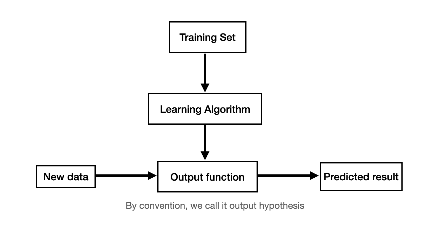
when design a linear regression algorithm, you may ask yourself the following questions
How to represent the output hypothesis?
In machine learning, linear regression hypothesis should be in form of $h(x) = a_0 + a_1x$
when the input $x$ is multi-dimension: $h(x) = h(x_1 , x_2 , … ,x_n) = a_0+a_1x_1+a_2x_2 + … +a_nx_n $
matrix representation
$$
\text{parameter}\ \theta =
\begin{bmatrix}
a_0 , a_1 , …,a_n
\end{bmatrix}
$$$$
\text{feature} \ x = \begin{bmatrix}
1\
x_1\
…\
x_n
\end{bmatrix}
$$
1 | import numpy as np |
The main job of the algorithm is to choose the parameters let
$$
\frac{1}{2} \sum_{i=0}^m(h_{\theta}(x^{(i)}) - y^{(i)})^2 = \min(\frac{1}{2} \sum_{i=0}^m(h(x^{(i)}) - y^{(i)})^2)
$$- m is the number of training examples you have
- y is the correct value
- $x^{(i)},y^{(i)}$ means the $x, y$ of example $ i$
- $\frac{1}{2} $ is for the purpose to simplify the arithmetic, when you do derivation, you can cancel it out with the power
- $h_{\theta}$ means the paramters of this hypothesis is $\theta$
Gradient Descent
- Start with a random $\theta$ , for example
parameters = np.zeros((1,n)) - Keep changing $\theta$ to reduce $J(\theta) = \frac{1}{2} \sum_{i=0}^m(h_{\theta}(x^{(i)}) - y^{(i)})^2$
- Note that $J(\theta)$ is the total loss of all train samples !!!
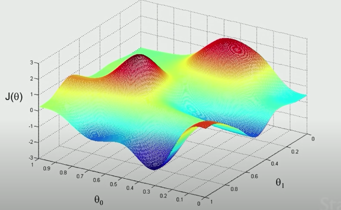
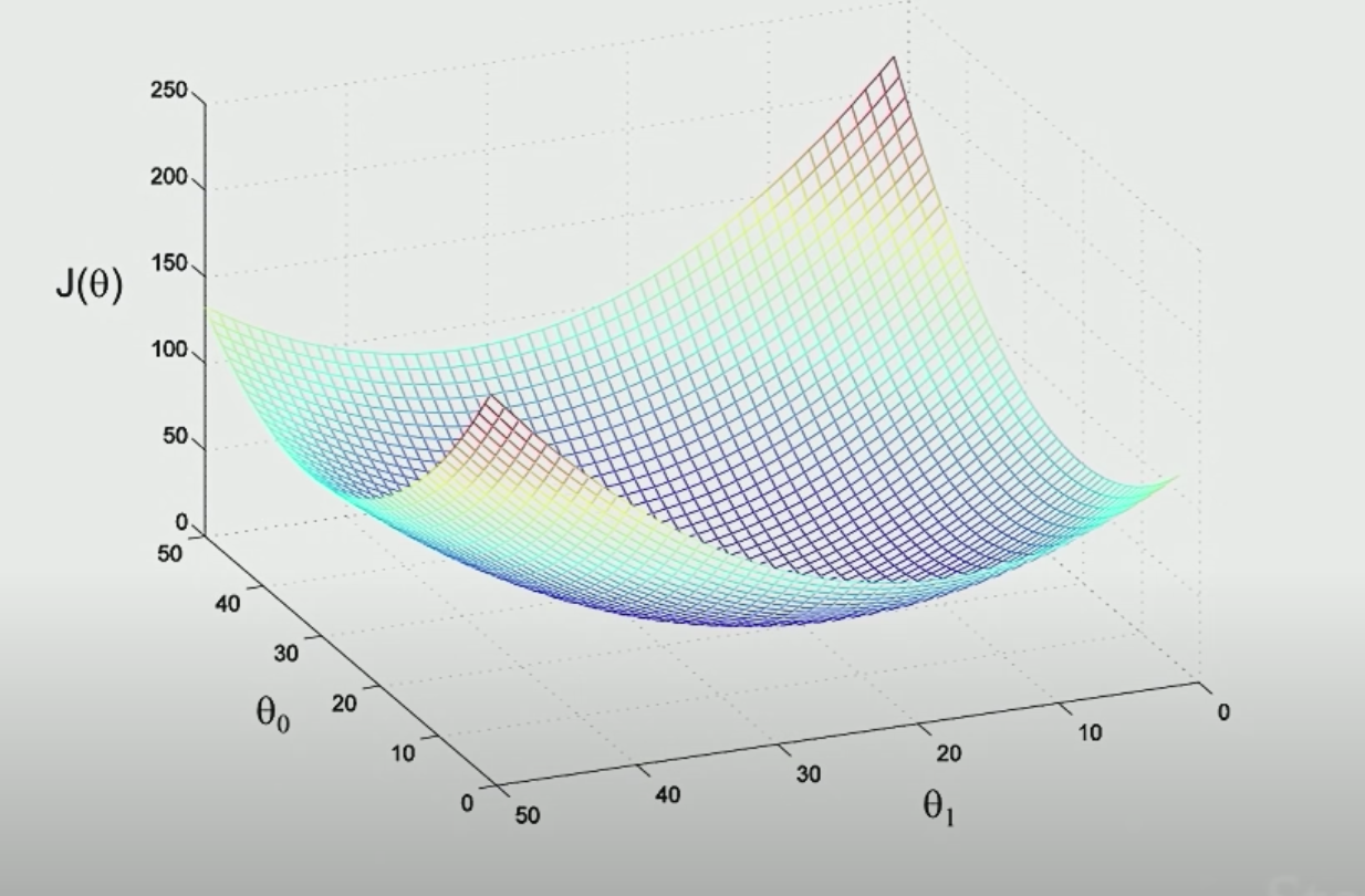
Example of 2-dimension x
add the $ J(\theta)$ as the extra dimension, calculate the values
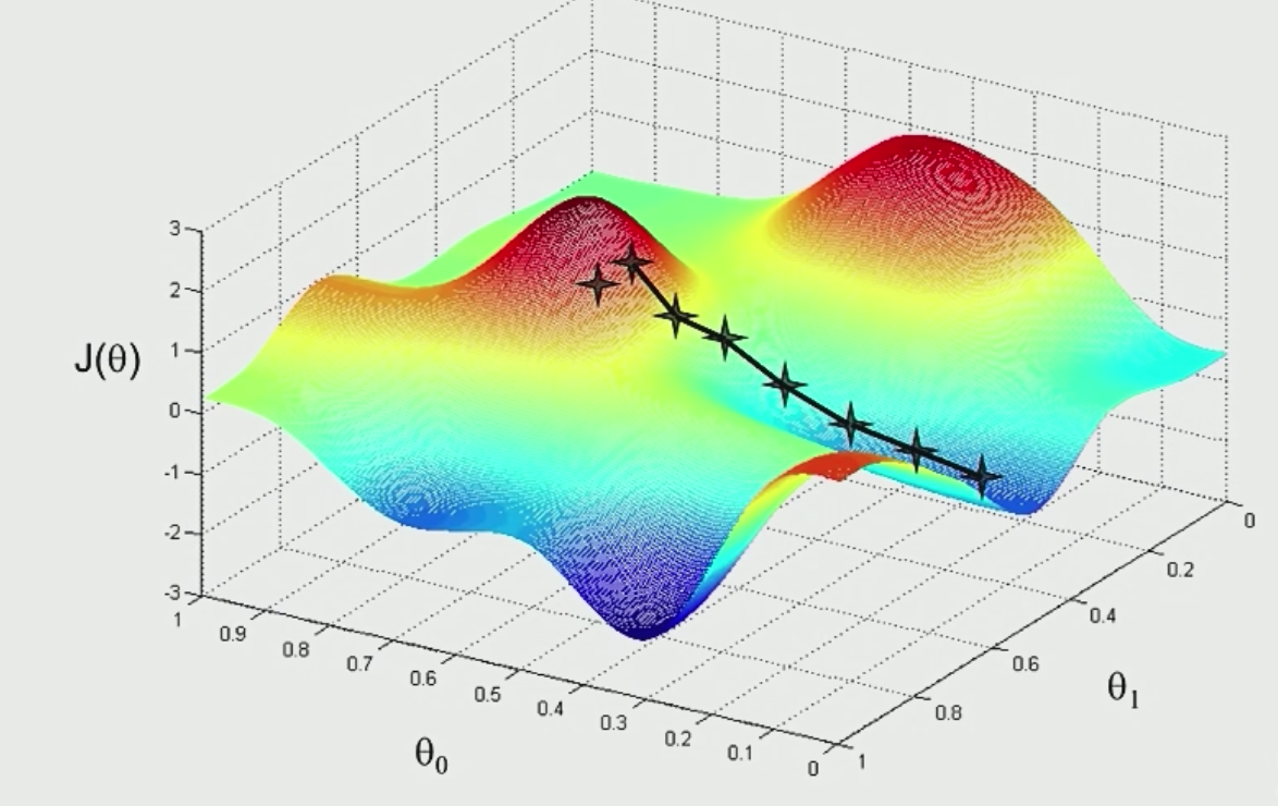
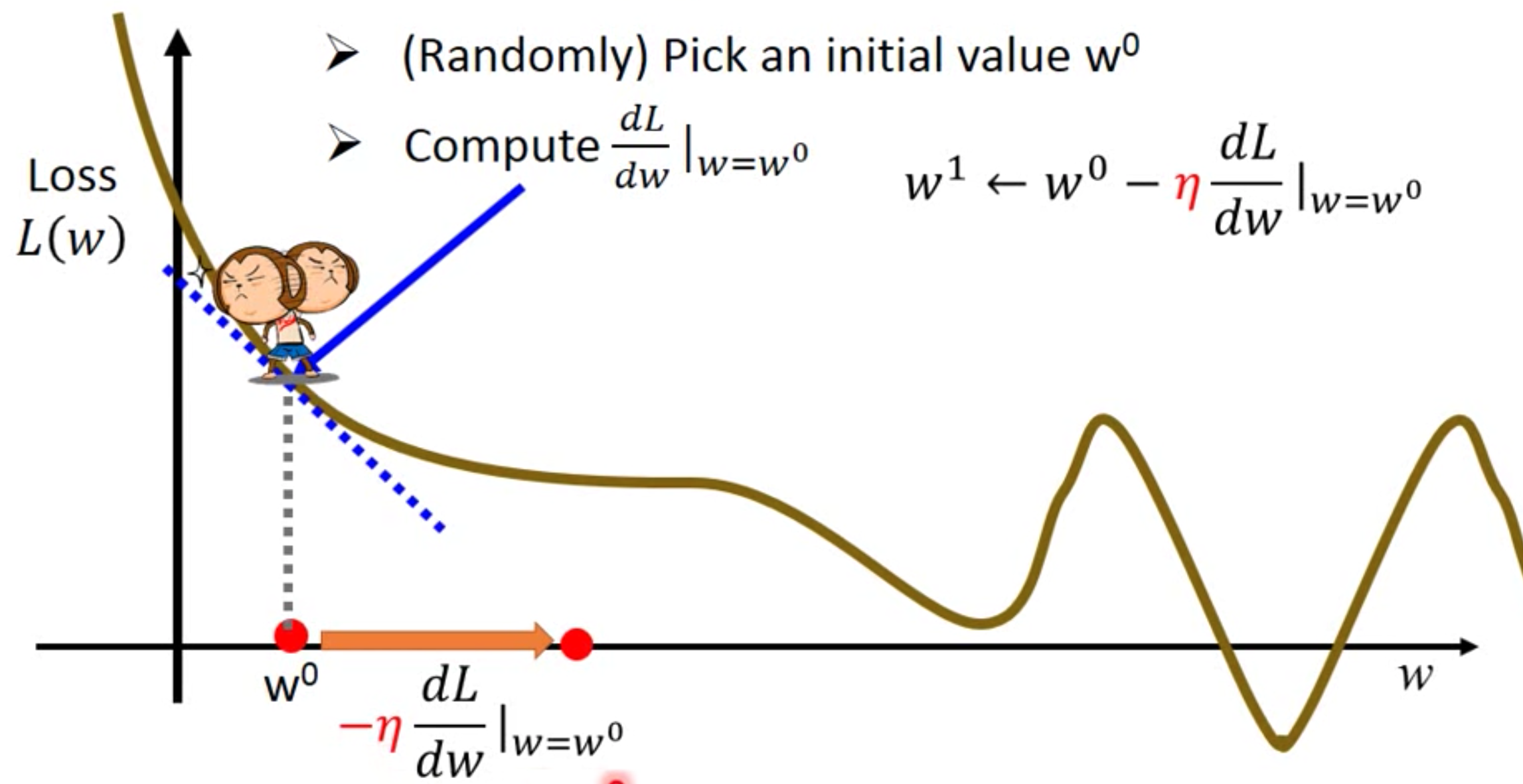
start from a random point, take a little step each time, follow the direction that decrease most(value of derivative is the least), you will reach a local minimum.
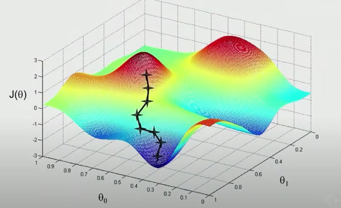
However, it is a local minimum, not a global one, so if you start from another random point, you may get a different result.
How to do the descending ?
update the parameters in each step
How to update?
move downwards, this picture show the section of one argument, explaining why we use -
$$
\theta_j := \theta_j - \alpha\frac{\partial(J(\theta))}{\partial\theta_j} (j=0,1,2,…,n)
$$
$$
\theta_j - \alpha\frac{\partial(J(\theta))} {\partial\theta_j} = \theta_j-\alpha[(h_\theta(x)-y)x_j]
$$
:=means assignment- $\alpha$ is the learning rate, it defines the ‘length’ of your each step, if it is too big, you may go beyond the mini point, see a increase in $\theta_j$, if it is too small, you have too wait for some time for the result to come out. So it is suggested that you can test several value of it, and then choose the most suitable one, like 0.01, 0.02, 0.04, 0.08, ……
in fact, you will have m training examples, so the forumla would be like
$$
\theta_j := \theta_j- \alpha \sum_{i=1}^m[h_\theta(x^{(i)})-y^{(i)}]x_j^{(i)} , (j=0,1,2,…n)
$$
also be called Repeat Until ConvergenceIt’s turn out that when using Linear Regression, and you define the loss function like $(y-x)^2, $ the picture will always look like a bowl, so the local minimum will be the global minimum, don’t worry.
Disadvantages
- The algorithm has to go over every training example in each upgrade, when the given data set is vary large, it will take vary vary long time to make a step, the amount of calculation is also quite big.(This algorithm is also called ‘Batch Gradient Descend’, and the ‘Batch’ means the the algorithm view all training examples as a ‘batch’. )
improve: Stochastic Gradient Descend
Instead of using every training example to make one upgrade, only use one example to make one upgrade
1 | while(1){ |
This is what it looks like:

- the algorithm will never converge, so you can stop it when you feel the output is comfortable to use.
- because your data set is very large, so you should have a bigger $\alpha$, too.
A trick especially for Linear Regression, Normal Equation
We can directly find out the value of θ without using Gradient Descent, only one step!
The big idea is that solve the equation, for what $\theta$, $\nabla_{\theta}J(\theta) = 0$
partial derivative for respect $\theta$
$$
\text{define} \nabla_{\theta}J(\theta) = \begin{bmatrix}
\frac{\partial J}{\theta_0}\
\frac{\partial J}{\theta_1}\
…\
\frac{\partial J}{\theta_n}\
\end{bmatrix}
$$partial matrix(two dimension as an example)
1
2
3
# say we have a function which maps a matrix to a real number.
def f(A:numpy.array):
return A[0][0] + A[0][1]$$
\text{then},\nabla_{A}f(A) = \begin{bmatrix}
\frac{\partial f}{A[0][0]} & \frac{\partial f}{A[0][1]}&…&\frac{\partial f}{A[0][n]}\
\frac{\partial f}{A[1][0]} & \frac{\partial f}{A[1][1]}&…&\frac{\partial f}{A[1][n]}\
… & …&…&…\
\frac{\partial f}{A[n][0]} & \frac{\partial f}{A[n][1]}&…&\frac{\partial f}{A[n][n]}\
\end{bmatrix}
$$
the output should be a matrix with the same dimension of Atrace of square matrix
$$
tr(A^{n\times n}) = \sum_{i=1}^nA_{ii}
$$Theorem 1:
1
2
3
def f(A:numpy.array):
B = numpy.array(.....) # B is some fixed matrix
return tr(AB)then
$$
\nabla_Af(A) = B ^{\mathbf{T}}
$$Theorem 2:
$$
tr(AB) = tr(BA)
$$
$$
tr(ABC) = tr(CAB)
$$
- Theorm 3:
$$
f(A) = tr(AA^{\mathbf{T}}C),\text{for some fixed C}
$$
then
$$
\nabla_Af(A) = CA+C^{\mathbf{T}}A
$$ - Design Matrix:
$$
X = \begin{bmatrix}
(x^{(1)})^{\mathbf{T}}\
(x^{(2)})^{\mathbf{T}}\
…\
(x^{(m)})^{\mathbf{T}}\
\end{bmatrix}
\
Y=\begin{bmatrix}
y^{(1)}\
y^{(2)}\
…\
y^{(m)}\
\end{bmatrix}
$$
then
$$
X\theta = \begin{bmatrix}
(x^{(1)})^{\mathbf{T}} \theta\
(x^{(2)})^{\mathbf{T}}\theta\
…\
(x^{(m)})^{\mathbf{T}}\theta\
\end{bmatrix} = \begin{bmatrix}
h_\theta(x^{(1)})\
h_\theta(x^{(2)})\
…\
h_\theta(x^{(m)})\
\end{bmatrix}
$$
then
$$
J(\theta) = \frac{1}{2} (X\theta-Y)^{\mathbf{T}} (X\theta-Y)
$$
$$
= \frac{1}{2}(\theta^{\mathbf{T}} X^{\mathbf{T}} - Y^{\mathbf{T}})(X\theta-Y)
$$
$$
=\frac{1}{2}(\theta^{\mathbf{T}} X^{\mathbf{T}} X\theta-\theta^{\mathbf{T}} X^{\mathbf{T}}Y-Y^{\mathbf{T}}\theta^{\mathbf{T}} X^{\mathbf{T}}+Y^{\mathbf{T}}Y)
$$
use theorems to simplify
$$
=\frac{1}{2} *2(X^{\mathbf{T}} X\theta - X^{\mathbf{T}}Y)
$$
$$
=X^{\mathbf{T}} X\theta - X^{\mathbf{T}}Y
$$
$$
\therefore \nabla_\theta J(\theta) = \nabla_\theta(X^{\mathbf{T}} X\theta - X^{\mathbf{T}}Y)
$$
$$
\text{let} \nabla_\theta J(\theta) =0
$$
$$
\therefore X^{\mathbf{T}} X\theta - X^{\mathbf{T}}Y =0
$$
$$
\therefore X^{\mathbf{T}} X\theta =X^{\mathbf{T}}Y
$$
$$
\therefore \theta = (X^{\mathbf{T}}X)^{-1}X^{\mathbf{T}}Y
$$