Locally Weighted Regression

Two type of learning algorithm

• Parametric learning Algorithm
  • fit fixed set of parameters to data
• Non-parametric learning algorithm
  • amount of data/parameters you need to keep grow with the size of data
  • Locally weighted Regression belongs to this type

High level preview of Locally weighted regression

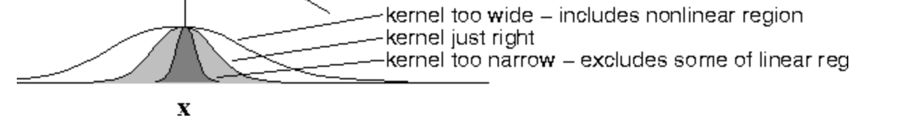
Fit $\theta$ to minimum the loss function $\sum_{i=1}^m w_i (y^{i} - \theta^{i}x^{i})^2$, where $w_i$ is a “weight” function, usually $w_i$ is given by the following:
$$
w_i = e^{-\frac{(x^{(i)}-x)^2}{2\tau^2}}
$$
which means
$$
\begin{cases}
w_i\longrightarrow1,&|x^{(i)}-x|\longrightarrow0\
w_i\longrightarrow0,&|x^{(i)}-x|\longrightarrow \infin
\end{cases}
$$
the more x is close to the training sample $x^{(i)}$, the more important $x^{(i)}$ will be

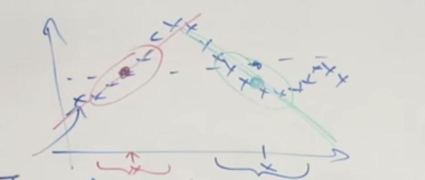
• we try to use only training sample near $x$ to make our predication

• you can control the “attention” span by changing the parameter $\tau$

  

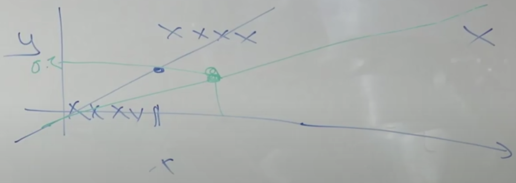
Classification Problem

Binary Classification

$$
y\in{0,1}
$$

Note that Linear Regression is absolutely NOT a good algorithm for Classification problem becasue classification problem has nothing to do with linear relationship!!!

We solve this kind of problem via Logistic Regression

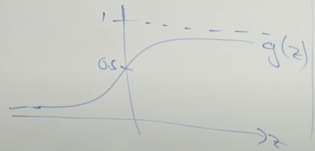
we want out hypothesis works like
$$
h(\theta) \in [0,1]
$$
so we have a logistic function
$$
g(z) = \frac{1}{1+e^{-z}} \in [0,1]
$$

we then feed our old linear regression hypothesis in to it to just reduce the value to [0,1]
$$
h(\theta) = g(\theta^Tx) = \frac{1}{1+e^{-\theta^Tx}}
$$
After some sophisticated math, we make a function which gives us the likelihood of our parameters now are the right ones, we call it a “log function”
$$
\log(\theta) = \sum_{i=1}^m y^{(i)} \log{h_\theta(x^{(i)})}+(1-y^{(i)})\log(1-h_\theta (x^{(i)}))
$$
becasue y is either 0 or 1, so it function like a switcher

Finally, we come with our solution : Gradient Ascent

compared with gradient descent, we try to maximum the correct probability.

update parameters in gradient ascent:
$$
\theta_j = \theta_j + \alpha \frac{\partial \log{(\theta)}}{\partial\theta_j}\
= \theta_j + \alpha \sum_{i=1}^m (y^{(i) } - h_\theta(x^{(i)}))x_j^{(i)}
$$
update parameters in gradient descent:
$$
\theta_j = \theta_j - \alpha \frac{\partial h (\theta)}{\partial\theta_j}
$$

• just like the gradient descent, gradient ascent has a local maximun same as global maximum
• No one shoot method like normal equation for gradient ascent
• but we have Newton’s method to accelerate

Newton’s method

give a function $f(\theta)$, Newton’s method try to find a $\theta$ that makes $f(\theta) = 0$

we can just set $f(\theta)$ to our $\log’(\theta)$ to find the $\theta$ that make max $\log (\theta)$

Here is how Newton’s method work

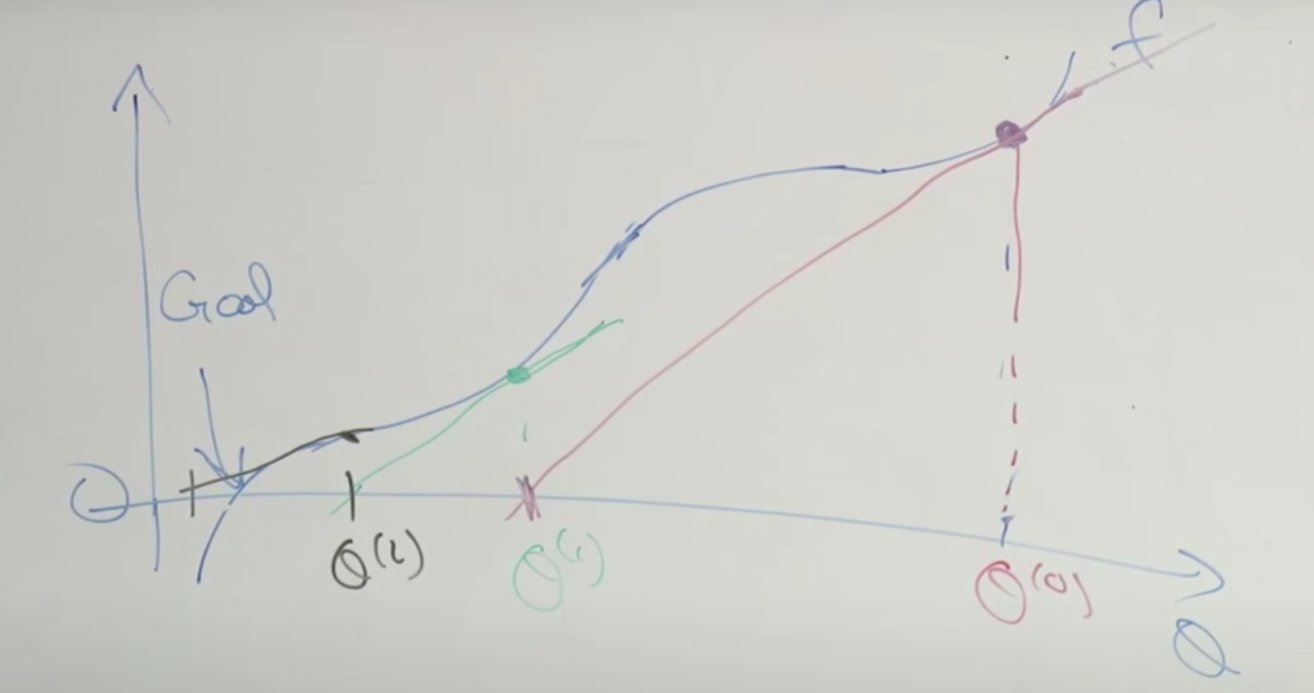
1. We start from a random $\theta_0$
2. Calculate the tangent line at $\theta_0$
3. let tangent line to be 0 to find $\theta_1$
4. Repeat until we find our target

Derivate the formula

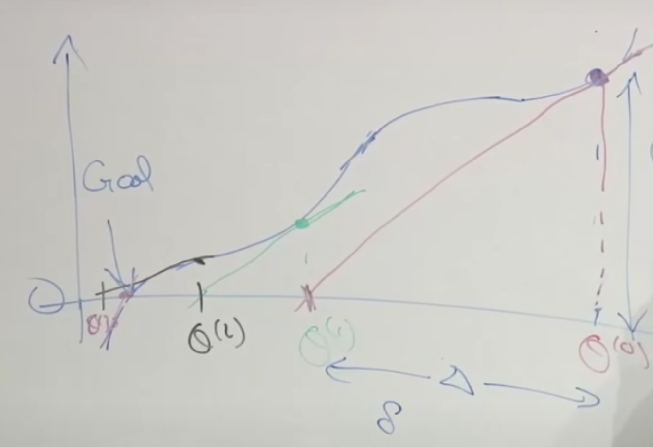
$$
\theta^{(1) } = \theta^{(0)} - \triangle
$$

$$
f’(\theta^{(0)}) = \frac{f(\theta_0)}{\triangle}
$$

$$
\theta^{(1) } = \theta^{(0)} - \frac{f(\theta_0)}{f’(\theta^{(0)})}
$$

$$
\theta^{(i+1)} = \theta^{(i)} - \frac{f(\theta_i)}{f’(\theta^{(i)})}
$$

Disadvantages

each step in newton’ method require to inverse a matrix, if number of your parameters is small, that’s fine. However, when you have many parameters, the dimension of your matrix is very high, each step will cost much.