Optimizing Program Performance
Writing an efficient program requires several types of activities
select an appropriate set of algorithms and data structures
write source code that the compiler can effectively optimize to turn into efficient executable code
divide a task into portions that can be computed in parallel, on some combination of multiple cores and multiple processors
( Even when exploiting parallelism, it is important that each parallel thread execute with maximum performance)
In general, programmers must make a trade-off between how easy a program is to implement and maintain, and how fast it runs
(For example simple bubble sort vs quick sort)
(For example optimizations will reduce readability)
When optimizing the program, the programmer work together with the compiler
Programmers should eliminate unnecessary work, making the code perform its intended task as efficiently as possible.(Reduce function call, memory reference ….)
To maximize the performance, a model of the target machine is very important.
How instructions are executed on the target machine is vital
(For example, the compiler need these information to decide it should choose to generate a mulitplication instruction or a combination of addition and shifting)
(On some machines, we can even perform an instruction-level parallelism, executing multiple instructions simultaneously)
Optimization can be a difficult job
- Performance can depend on many detailed features of the processor design for which we have relatively little documentation or understanding
- It can be difficult to explain exactly why a particular code sequence has a particular execution time.
- So optimization is not a linear job of transfering code by applying several rules (as we will do), but it is a lot of trial-and-error experimentation is required.
It might seem strange to keep modifying the source code in an attempt to coax the compiler into generating efficient code, but this is indeed how many high-performance programs are written.
5.1 Capabilities and Limitations of Optimizing Compilers
Compilers must be careful to apply only safe optimizations to a program
For example
1 | void twiddle1(long *xp, long *yp) |
- These two functions are seemingly same
twiddle2will be more efficient thantwiddle1since it only refers the memory for 3 times rather than 4 times- However, if
xp == yp,twiddle1will gives4 * (*xp)whiletwiddle2gives3 * *(*xp) - So the complier don’t know how the function will be called, so it cannot generate optimized code based on
twiddle2fortwiddle1
The case where two pointers may designate the same memory location is known as ==memory aliasing==, which is a major optimization blockers, preventing compiler from applying some optimization
Another example
1 | x = 1000; y = 3000; |
Practice Problem 5.1
The following problem illustrates the way memory aliasing can cause unexpected program behavior. Consider the following procedure to swap two values:
2
3
4
5
6
{
*xp = *xp + *yp; /* x+y */
*yp = *xp - *yp; /* x+y-y = x */
*xp = *xp - *yp; /* x+y-x = y */
}If this procedure is called with xp equal to yp, what effect will it have?
My solution:
1 |
|
A second optimization blocker is due to ==function calls==.
1 | long f(); |
func1callf4 times whilefunc2callfonly onceAgain the compiler cannot optimize
func1intofunc2An hazard example
1
2
3
4long globaldata = 0;
f(){ return globaldata++ ;}
//func1() = 0 + 1 + 2 + 3 == 6
//func2() = 0 * 4 == 0Code involving function calls can be optimized by a process known as inline substitution, where the function call is replaced by the code for the body of the function(some compiler will do this, but
gccwon’t)
5.2 Expressing Program Performance
We introduce the metric cycles per element, abbreviated CPE, to express program performance in a way that can guide us in improving the code
For example, here are some codes for computation the prefix-sum of a float vector
1 | /* Compute prefix sum of vector a */ |
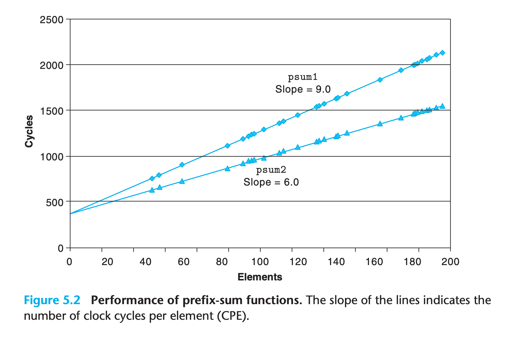
The performance can be fit into a linear module of y = kx + b
bis the time used to initialized the loopkis what we called CPE(how many clocks are needed to operate on one element)
Practice Problem 5.2
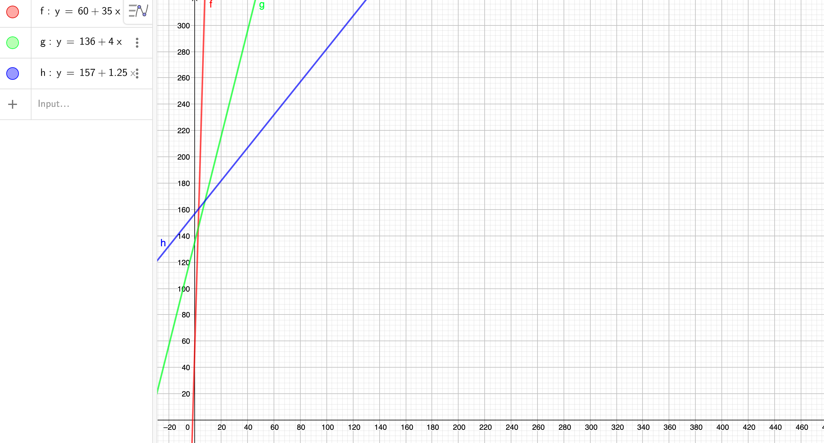
Later in this chapter we will start with a single function and generate many different variants that preserve the function’s behavior, but with different performance characteristics. For three of these variants, we found that the run times (in clock cycles) can be approximated by the following functions:
2
3
Version 2: 136 + 4n
Version 3: 157 + 1.25nFor what values of n would each version be the fastest of the three? Remember that n will always be an integer
My solution : :white_check_mark:
(Graph drawn by geogebra)
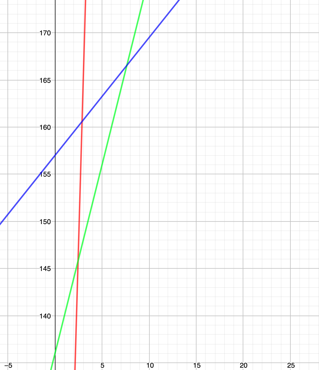
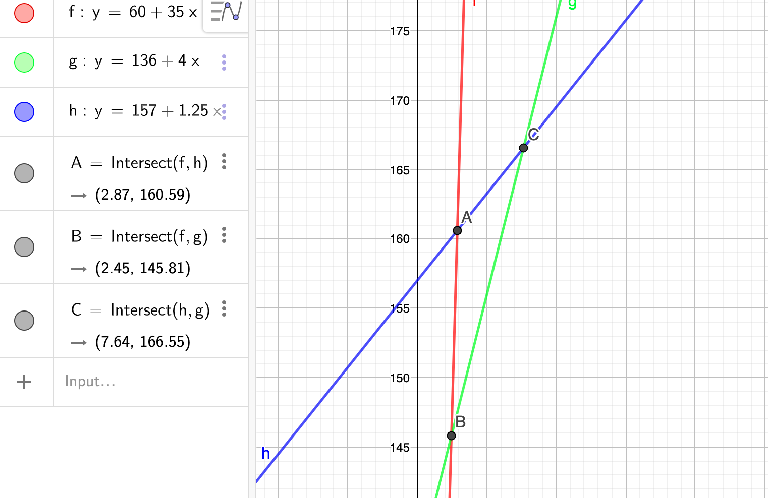
Let’s zoom in and do some math
$$
60 + 35x \le 136 + 4x
$$
$$
x \le \frac{76}{31}
$$
$$
\because x \in Z^+
$$
$$
\therefore x \le 2
$$
when x less equals than 2, version 1 consume the leatest time
The rest are the same
$$
\therefore \text{fastest version } = \begin{cases}
1 , & 0 \le x \le 2\
2 , & 3 \le x\le 7 \
3 , & x \ge 8
\end{cases}
$$
5.3 Program Example
To demonstrate how an abstract program can be systematically transformed into more efficient code, we will use a running example based on the vector data structure
1 | /* Create abstract data type for vector */ |
We want to test multiple date type and different operations in C
1 | typedef long /* int , float , double */ data_t; |
Example program code
1 | /* Create vector of specified length */ |
In our experience, the best approach involves a combination of experimentation and analysis:
repeatedly attempting different approaches, performing measurements, and examining the assembly-code representations to identify underlying performance bottlenecks.
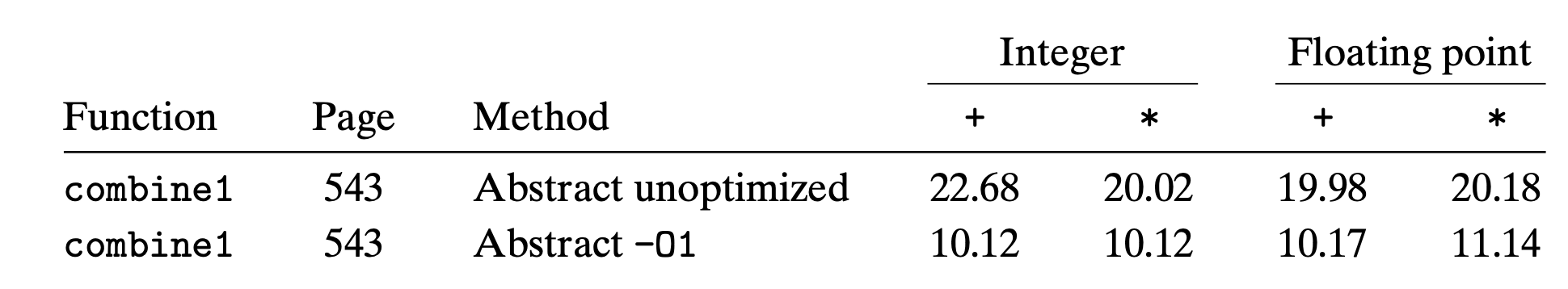
Run time of combine1
- use
chrtto give your program high priority - install
perf - Why
perfhave some value unsupported in VM perfdepend on Linux specified code, so it isn’t available to MacOS- Linux
aptreportCould not get lock /var/lib/dpkg/lock-frontend - open
Finally I had to use /usr/bin/time --verbose /path/to/program to measure the performance
5.4 Eliminating Loop Inefficiencies
Oberserve that the length of vector doesn’t change during the loop, we can eliminate the function call of vec_length to reduce some instructions.
We modify combine1 as what we described above to get combine2
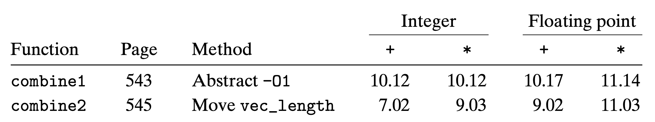
This optimization is an instance of a general class of optimizations known as code motion
- They involve identifying a computation that is performed multiple times(within a loop) but the result don’t change
- We can therefore move the computation to an earlier section of the code that does not get evaluated as often.
You think you won’t write codes like this ? Here is a very practical example.
1 | /* Convert string to lowercase: slow */ |
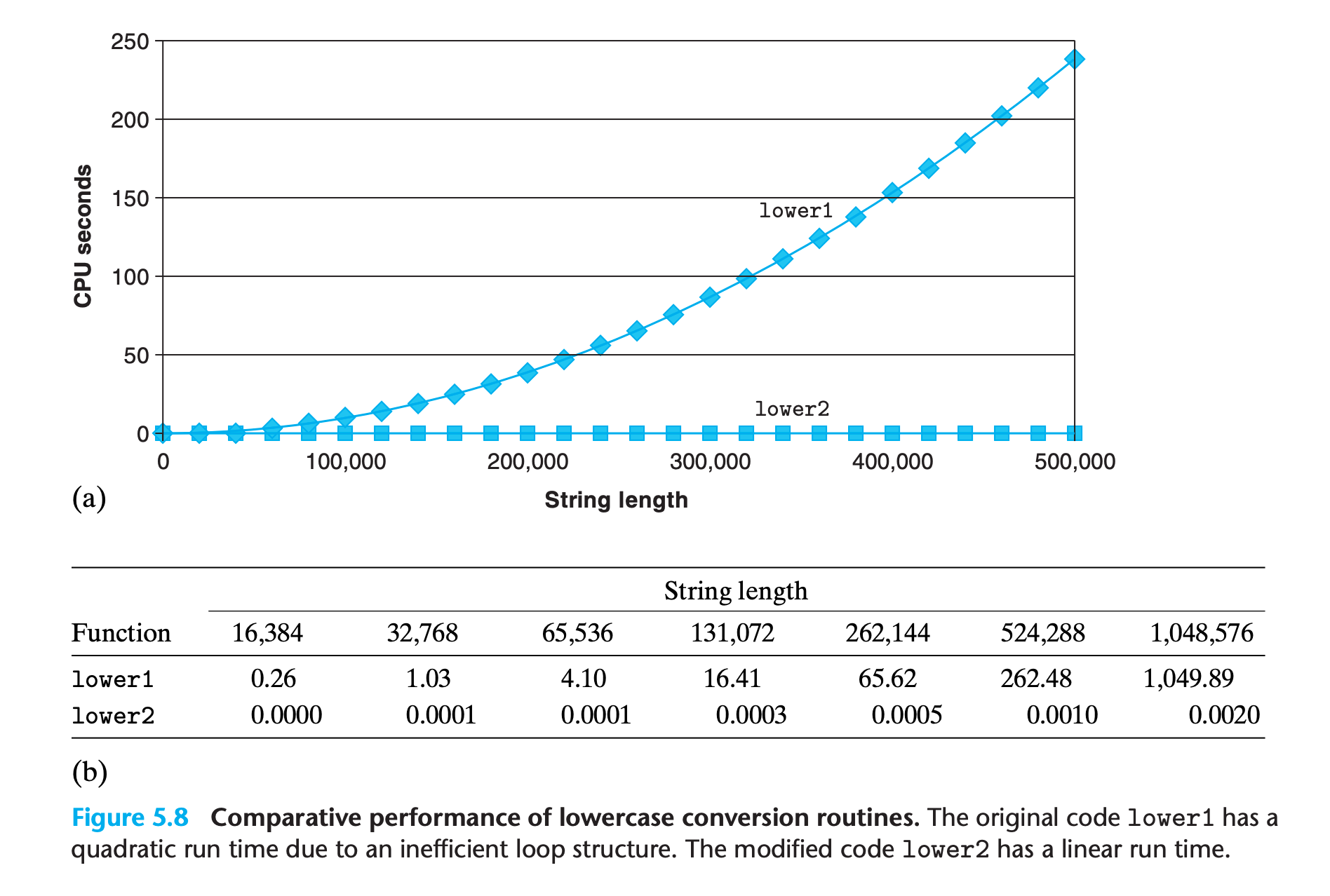
The compiler can’t do optimization for you in this case, since it need to know that even the content of string was changed the length of it will not. Even the most sophisticated compiler is unqualified.
Part of the job of a competent programmer is to avoid ever introducing such asymptotic inefficiency
Practice Problem 5.3
Consider the following functions:
2
3
4
long max(long x, long y) { return x < y ? y : x; }
void incr(long *xp, long v) { *xp += v; }
long square(long x) { return x*x; }The following three code fragments call these functions:
2
3
4
5
6
7
8
t += square(i);
B. for (i = max(x, y) - 1; i >= min(x, y); incr(&i, -1))
t += square(i);
C. long low = min(x, y);
long high = max(x, y);
for (i = low; i < high; incr(&i, 1))
t += square(i);Assume x equals 10 and y equals 100.
Fill in the following table indicating the number of times each of the four functions is called in code fragments A–C:
Code min max incr square A B C
My solution : :white_check_mark:
Beware that the function used as condition will be call one more time when quiting the loop
| Code | min | max | incr | square |
|---|---|---|---|---|
| A | 1 | 91 | 90 | 90 |
| B | 91 | 1 | 90 | 90 |
| C | 1 | 1 | 90 | 90 |
The subtle difference is critical to performance
1 |
|
5.5 Reducing Procedure Calls
We can see in the code for combine2 that get_ vec_element is called on every loop iteration to retrieve the next vector element.
- A simple analysis of the code for combine2 shows that all references will be valid, so we can remove bound check
- Rather than making a function call to retrieve each vector element, we can accesses the array directly
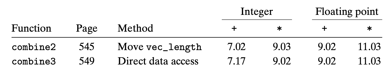
However, performance doesn’t improve at all!
- The modification we have made is not wise
- In principle, the user of the vector abstract data type should not even need to know that the vector contents are stored as an array, rather than as some other data structure such as a linked list.
- A purist might say that this transformation seriously impairs the program modularity
So why would this happen? See 5.11.2
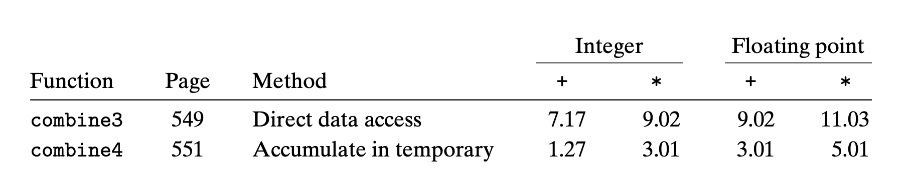
5.6 Eliminating Unneeded Memory References
In combine3
1 | void combine3(vec_ptr v, data_t *dest) |
We can see that memory pointed by dest are referred mulitple times
1 | #Inner loop of combine3. data_t = double, OP = * |
This reading and writing is wasteful, since the value read from dest at the beginning of each iteration should simply be the value written at the end of the previous iteration
We should use a temp variable(a register) to accumulate the value
1 | #Inner loop of combine4. data_t = double, OP = * |
1 | /* Accumulate result in local variable */ |
Again, the compiler cannot optimize the code automatically, since the hazard of memory alias. For example
1 | v = [2,3,4]; |
Practice Problem 5.4
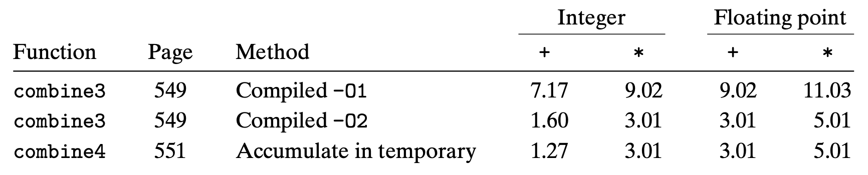
When we use gcc to compile combine3 with command-line option -O2, we get code with substantially better CPE performance than with -O1:
We achieve performance comparable to that for combine4, except for the case of integer sum, but even it improves significantly. On examining the assembly code generated by the compiler, we find an interesting variant for the inner loop:
2
3
4
5
6
7
8
9
#dest in %rbx, data+i in %rdx, data+length in %rax
#Accumulated product in %xmm0
.L22: loop:
vmulsd (%rdx), %xmm0, %xmm0 #Multiply product by data[i]
addq $8, %rdx #Increment data+i
cmpq %rax, %rdx #Compare to data+length
vmovsd %xmm0, (%rbx) #Store product at dest
jne .L22 #If !=, goto loopWe can compare this to the version created with optimization level 1:
2
3
4
5
6
7
8
9
#dest in %rbx, data+i in %rdx, data+length in %rax
.L17: loop:
vmovsd (%rbx), %xmm0 #Read product from dest
vmulsd (%rdx), %xmm0, %xmm0 #Multiply product by data[i]
vmovsd %xmm0, (%rbx) #Store product at dest
addq $8, %rdx #Increment data+i
cmpq %rax, %rdx #Compare to data+length
jne .L17 #If !=, goto loopWe see that, besides some reordering of instructions, the only difference is that the more optimized version does not contain the
vmovsdimplementing the read from the location designated bydestA. How does the role of register
%xmm0differ in these two loops?B. Will the more optimized version faithfully implement the C code of
combine3, including when there is memory aliasing between dest and the vector data?C. Either explain why this optimization preserves the desired behavior, or give an example where it would produce different results than the less optimized code.
My solution : :white_check_mark:
A:
In combine3 -O2, %xmm0 serves as the result of each iteration
In combine3 -O1, %xmm0 serves as the read destination.
B:
Yes
C:
Because the optimized code actually do the write back, keeping the value at dest up-to-date
5.7 Understanding Modern Processors
One of the remarkable feats of modern microprocessors is that they employ complex and exotic microarchitectures, in which multiple instructions can be executed in parallel, while presenting an operational view of simple sequential instruction execution.(Called instruction-level-parallelism)
We will find that two different lower bounds characterize the maximum performance of a program
- Latency
- Throughput
5.7.1 Overall Operation
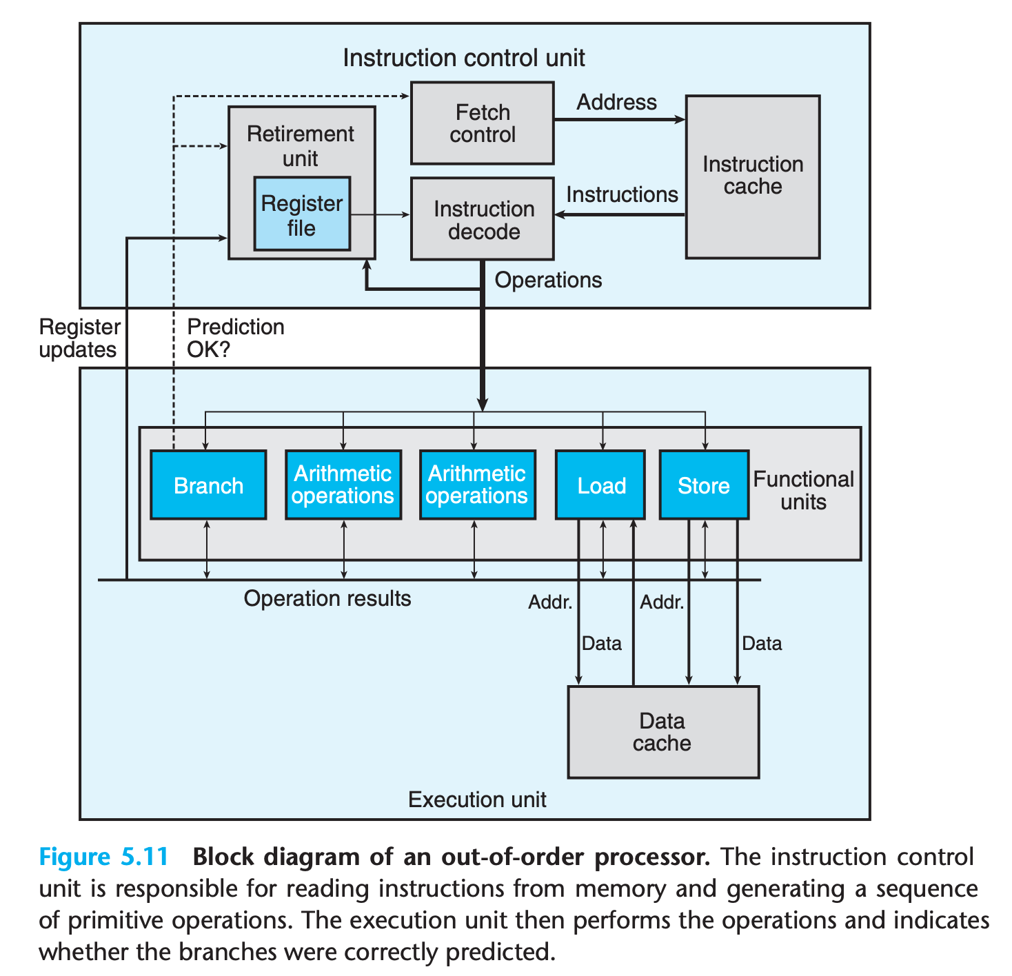
The overall design has two main parts:
The instruction control unit (ICU), which is responsible for reading a sequence of instructions from memory and generating from these a set of primitive operations(sometimes referred to as micro-operations) to perform on program data
1
2
3
4
5
6
7# For complex instruction machine
addq %rax,%rdx -> a simple add operation
addq %rax,8(%rdx) -> three micro-operations
-> read from memory M[8+%rdx]
-> addition
-> store the result to memoryThe execution unit (EU), which then executes these operations.
Compared to the simple in-order pipeline we studied in Chapter 4, out-of-order processors require far greater and more complex hardware, but they are better at achieving higher degrees of instruction-level parallelism.
Within the ICU, the retirement unit keeps track of the ongoing processing and makes sure that it obeys the sequential semantics of the machine-level program.
- Once the operations for the instruction have completed and any branch points leading to this instruction are confirmed as having been correctly predicted, the instruction can be retired, with any updates to the program registers being made.
- If some branch point leading to this instruction was mispredicted, on the other hand, the instruction will be flushed, discarding any results that may have been computed. By this means, mispredictions will not alter the program state.
Also, a technique call register renaming is used to implement function like data-forwarding
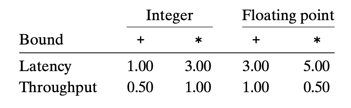
5.7.2 Functional Unit Performance
Hardware limit the ultimate performance of programs
5.7.3 An Abstract Model of Processor Operation
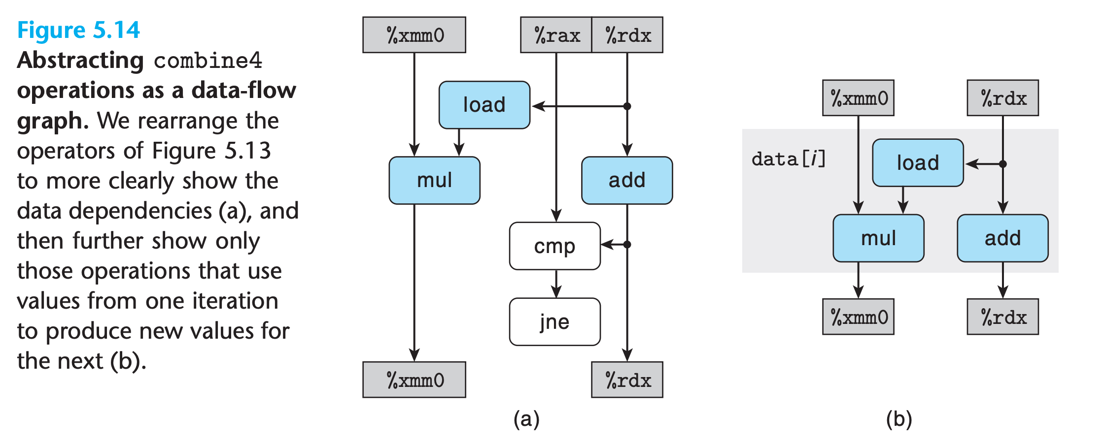
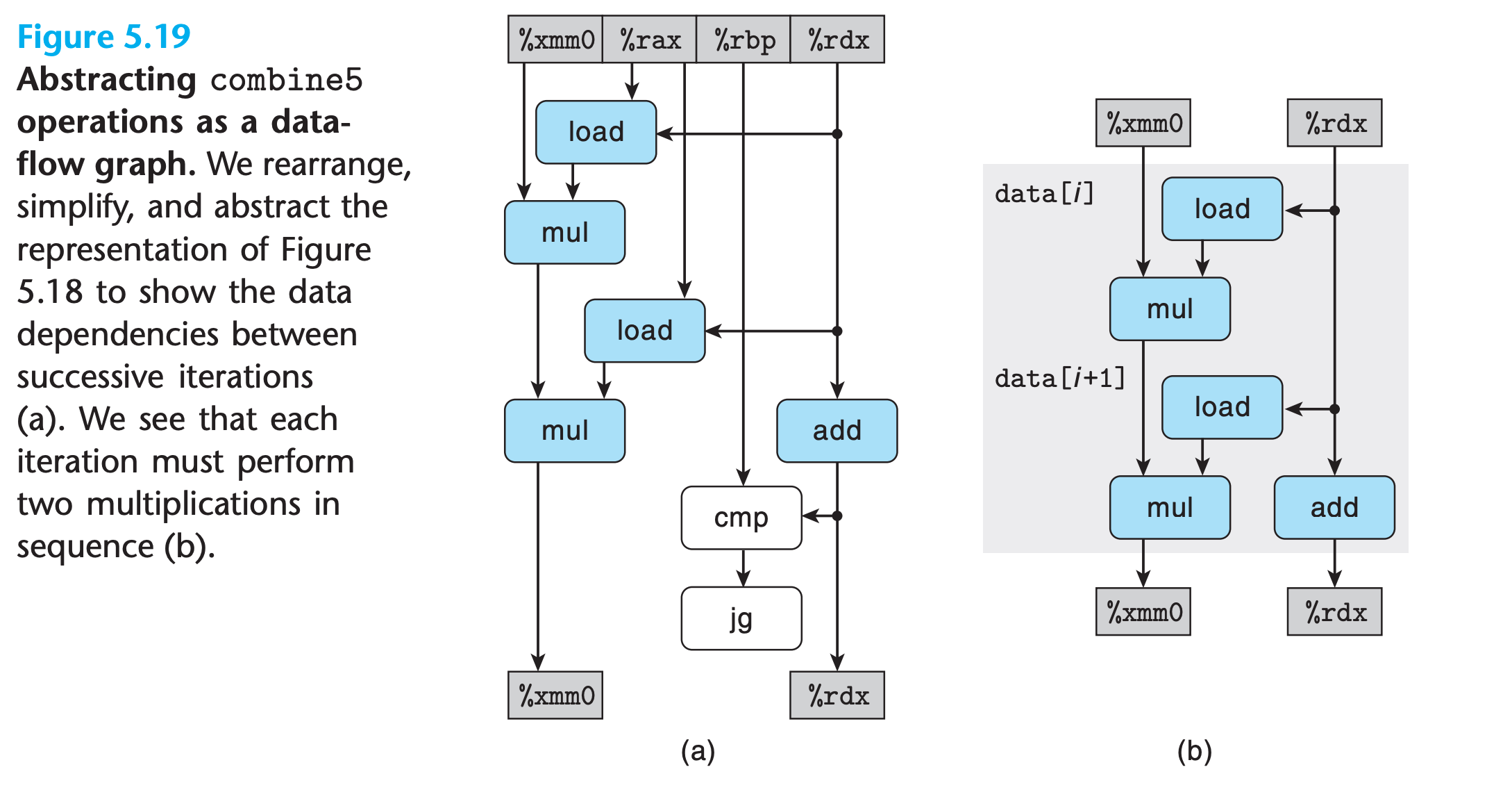
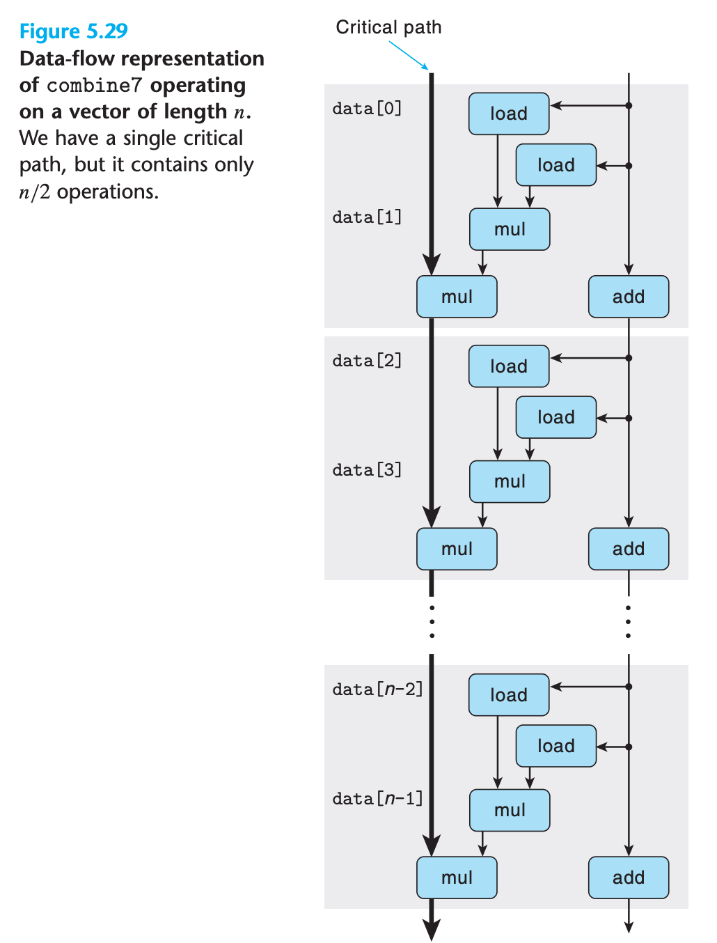
we will use a data-flow representation of programs, a graphical notation showing how the data dependencies between the different operations constrain the order in which they are executed
These constraints then lead to critical paths in the graph, putting a lower bound on the number of clock cycles required to execute a set of machine instructions.
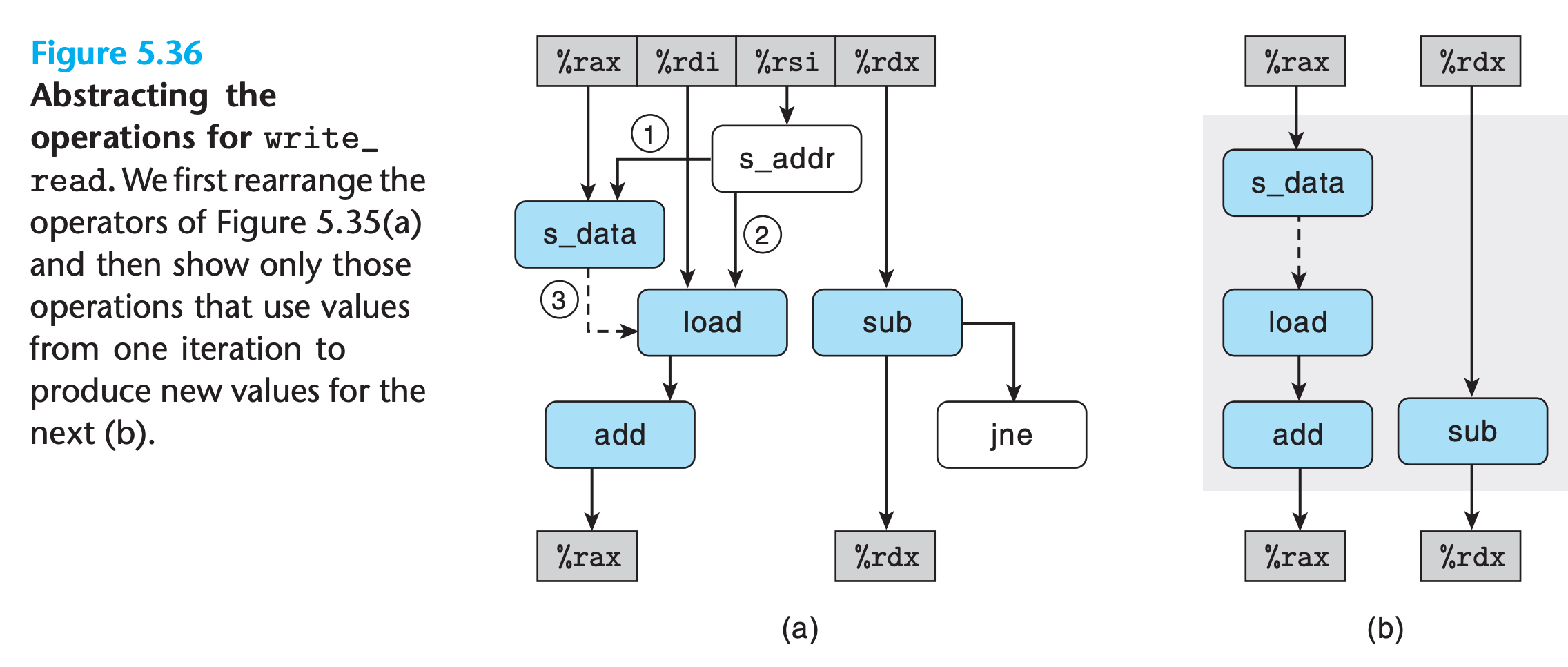
From Machine-Level Code to Data-Flow Graphs
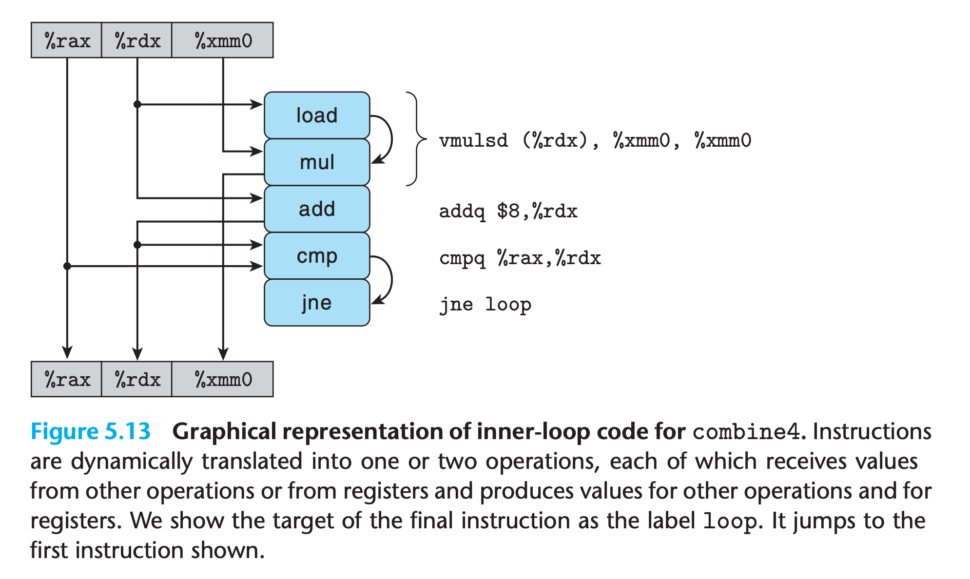
The registers at top store values before execution, those at the bottom store values after execution
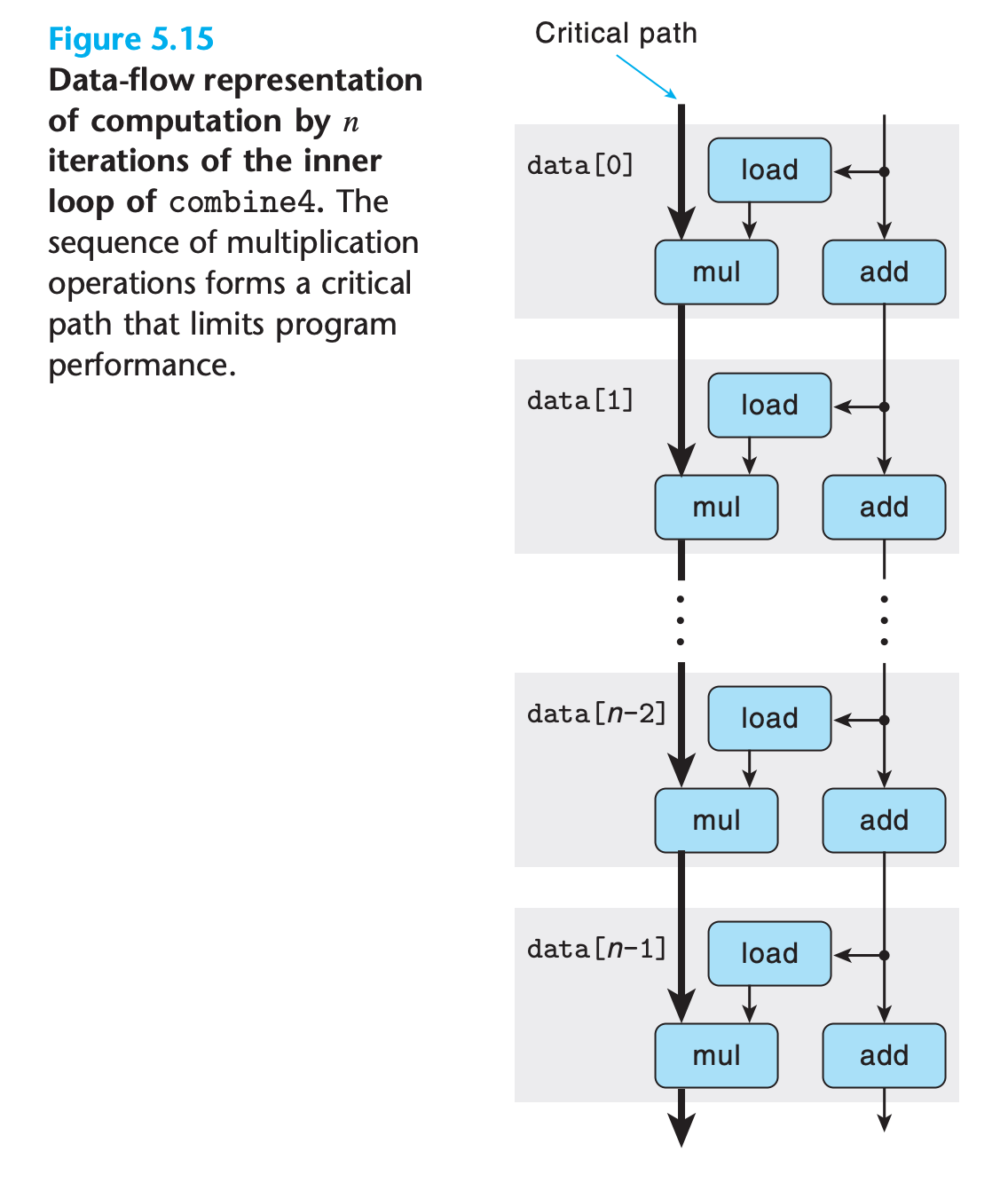
The left chain needs 5n clocks while the right chain needs only n clocks
So when executing the function, the floating-point multiplier becomes the limiting resource.
The other operations required during the loop—manipulating and testing pointer value data+i and reading data from memory—proceed in parallel with the multiplication. As each successive value of acc is computed, it is fed back around to compute the next value, but this will not occur until 5 cycles later
Other Performance Factors
Other factors can also limit performance, including the total number of functional units available and the number of data values that can be passed among the functional units on any given step.
Our next task will be to restructure the operations to enhance instruction-level parallelism. We want to transform the program in such a way that our only limitation becomes the throughput bound, yielding CPEs below or close to 1.00.
Practice Problem 5.5
Suppose we wish to write a function to evaluate a polynomial, where a polynomial of degree n is defined to have a set of coefficients $a_0, a_1, a_2,…,a_n$. For a value x, we evaluate the polynomial by computing
$$
a_0 + a_1x + a_2x_2 + … + a_nx_n
$$
This evaluation can be implemented by the following function, having as arguments an array of coefficients a, a value x, and the polynomial degree degree (the value n in Equation 5.2). In this function, we compute both the successive terms of the equation and the successive powers of x within a single loop:
2
3
4
5
6
7
8
9
10
11
{
long i;
double result = a[0];
double xpwr = x; /* Equals x^i at start of loop */
for (i = 1; i <= degree; i++) {
result += a[i] * xpwr;
xpwr = x * xpwr;
}
return result;
}A. For degree n, how many additions and how many multiplications does this code perform?
B. On our reference machine, with arithmetic operations having the latencies shown in Figure 5.12, we measure the CPE for this function to be 5.00. Explain how this CPE arises based on the data dependencies formed between iterations due to the operations implementing lines 7–8 of the function.
My solution :
A : n addition and 2n multiplication
B : the two multiplication can run in parallel
Solution on the book:
B. We can see that the performance-limiting computation here is the repeated computation of the expression xpwr = x * xpwr. This requires a floatingpoint multiplication (5 clock cycles), and the computation for one iteration cannot begin until the one for the previous iteration has completed. The updating of result only requires a floating-point addition (3 clock cycles) between successive iterations.
Practice Problem 5.6
$$
a_0 + x(a_1 + x(a_2 + … + x(a_{n−1} + xa_n) …))
$$Using Horner’s method, we can implement polynomial evaluation using the following code:
2
3
4
5
6
7
8
9
double polyh(double a[], double x, long degree)
{
long i;
double result = a[degree];
for (i = degree-1; i >= 0; i--)
result = a[i] + x*result;
return result;
}A. For degree n, how many additions and how many multiplications does this code perform?
B. On our reference machine, with the arithmetic operations having the latencies shown in Figure 5.12, we measure the CPE for this function to be 8.00. Explain how this CPE arises based on the data dependencies formed between iterations due to the operations implementing line 7 of the function.
C. Explain how the function shown in Practice Problem 5.5 can run faster, even though it requires more operations.
My solution :
A : n addition and n multiplication
B : addition must wait for multiplication to complete
C : in 5.5 the two multiplication can run in parallel
Solution on the book :
B. We can see that the performance-limiting computation here is the repeated computation of the expression result = a[i] + x*result. Starting from the value of result from the previous iteration, we must first multiply it by x (5 clock cycles) and then add it to a[i] (3 cycles) before we have the value for this iteration. Thus, each iteration imposes a minimum latency of 8 cycles, exactly our measured CPE.
C. Although each iteration in function poly requires two multiplications rather than one, only a single multiplication occurs along the critical path per iteration.
Verification :
“Better algorithm” does not guarantee a better performance !!!
Reduce data dependency really matters !!!
1 |
|
1 | $ for ((i = 0 ; i < 10 ; i++)) ./test |
(I once thought that it is the data cache resulted in the improvement, but reverse the order of function call gives the same result)
1 | Horner method cost : 0.002377 |
5.8 Loop Unrolling
Loop unrolling is a program transformation that reduces the number of iterations for a loop by increasing the number of elements computed on each iteration
Loop unrolling can improve performance in two ways
- It reduces the number of operations that do not contribute directly to the program result, such as loop indexing and conditional branching.
- We can further transform the code to reduce the number of operations in the critical paths of the overall computation.
k × 1 loop unrolling strategy
processing k elements in one loop
- upper limit to be
i < n − k + 1to prevent out-of-bound reference(fromitoi+k-1in each iteration,i+k-1 < n) - Loop index
iis incremented bykin each iteration - We include the second loop to step through the final few elements of the vector one at a time. The body of this loop will be executed between
0andk − 1times. - For example when
k == 2
1 | /* 2 x 1 loop unrolling */ |
Practice Problem 5.7 :white_check_mark:
Modify the code for combine5 to unroll the loop by a factor k = 5.
My solution :
1 | /* 5 x 1 loop unrolling */ |
Verification:
1 | time consumed by combine5 : 0.000861 |
(reverse function call order is done to ensure the improvement is not caused by cache)
Solution on the book does not solve data dependency either.
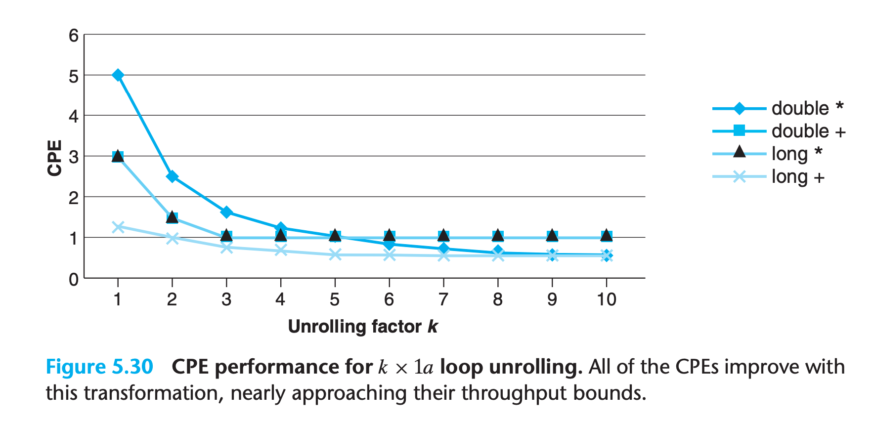
==Loop unrolling can easily be performed by a compiler==. Many compilers do this as part of their collection of optimizations. gcc will perform some forms of loop unrolling when invoked with optimization level 3 or higher
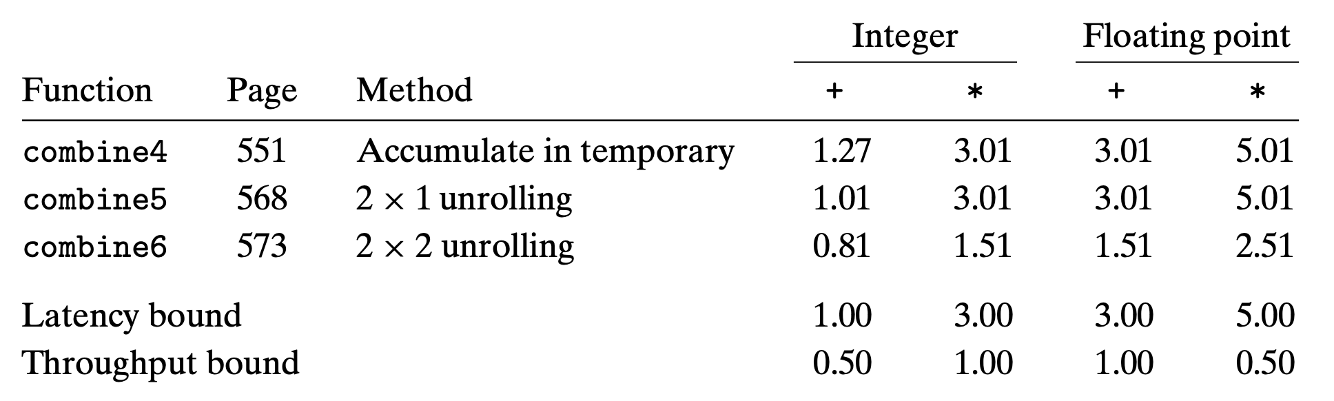
We see that the CPE for integer addition improves, achieving the latency bound of 1.00
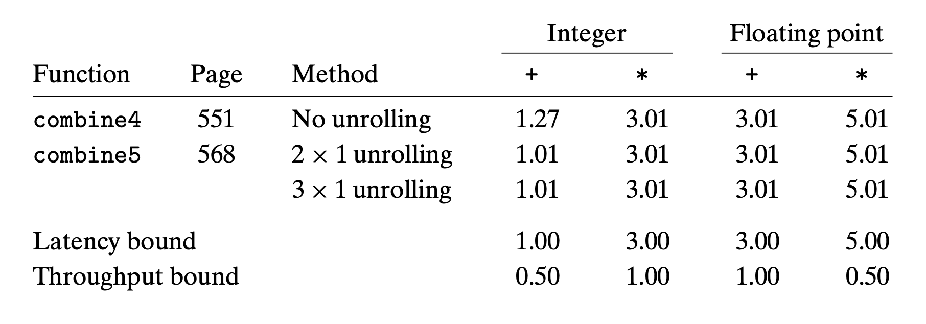
By reducing the number of overhead operations relative to the number of additions required to compute the vector sum, we can reach the point where the 1-cycle latency of integer addition becomes the performancelimiting factor.
On the other hand, none of the other cases improve—they are already at their latency bounds
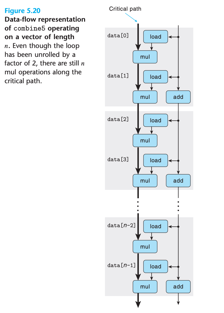
By examining the machine-level code, we can see that there is still a critical path of n multiplication operations —there are half as many iterations, but each iteration has two multiplication operations in sequence
5.9 Enhancing Parallelism
The functional units performing addition and multiplication are all fully pipelined, meaning that they can start new operations every clock cycle, and some of the operations can be performed by multiple functional units.
We will now investigate ways to break sequential dependency and get performance better than the latency bound.
5.9.1 Multiple Accumulators
For a combining operation that is ==associative and commutative==, such as integer addition or multiplication, we can improve performance by splitting the set of combining operations into two or more parts and combining the results at the end.
For example for n elements:
1 | result = n1 * n2 * n3 ... * n; |
We call this $2 \times 2 $ loop unrolling, 2 elements per iteration and 2 elements operate parallelly.
1 | /* 2 x 2 loop unrolling */ |
(I suppose the arithmetic result of floating point is not correct here)
The processor no longer needs to delay the start of one sum or product operation until the previous one has completed.
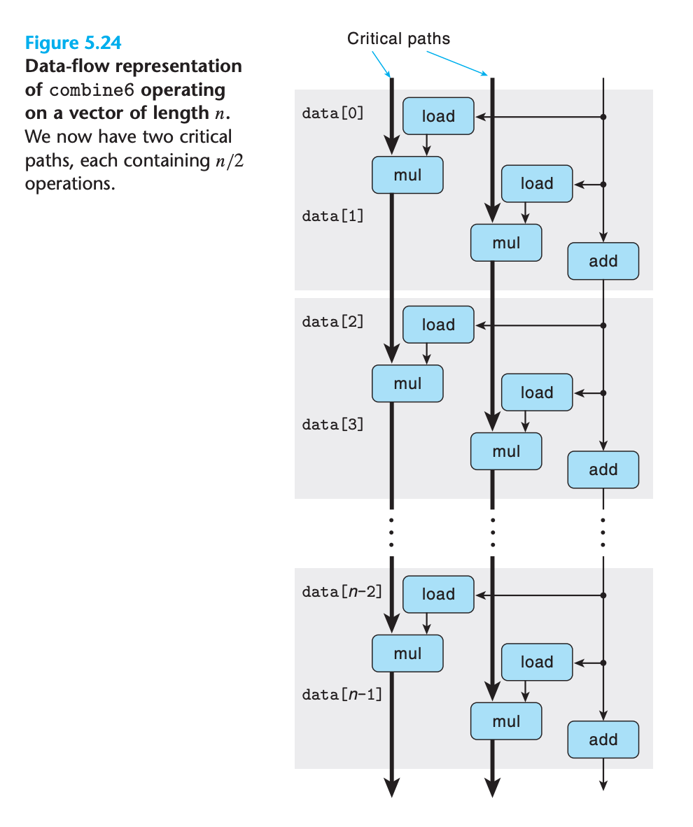
We see that we now have two critical paths run in parallel, so data dependency is reduced.
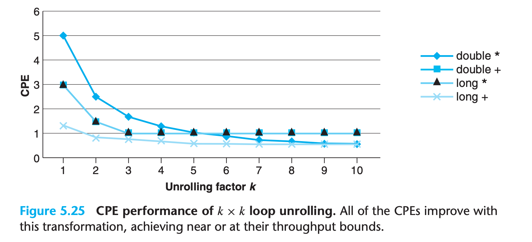
We can generalize the multiple accumulator transformation to unroll the loop by a factor of k and accumulate k values in parallel, yielding k × k loop unrolling.
We can see that, for sufficiently large values of k, the program can achieve nearly the throughput bounds for all cases.
In performing the k × k unrolling transformation, we must consider whether it preserves the functionality of the original function
We have seen in Chapter 2 that two’s-complement arithmetic is commutative and associative, even when overflow occurs.
Hence the compiler may apply this optimization strategy to the code
On the other hand, floating-point multiplication and addition are not associative. Thus, combine5 and combine6 could produce different results due to rounding or overflow.
So compilers won’t do this kind of transformation.
(In most real-life applications, however, such patterns are unlikely. Since most physical phenomena are continuous, numerical data tend to be reasonably smooth and well behaved)
( It is unlikely that multiplying the elements in strict order gives fundamentally better accuracy than does multiplying two groups independently and then multiplying those products together)
The programmer should decide whether they should make the trade-off or not.
5.9.2 Reassociation Transformation
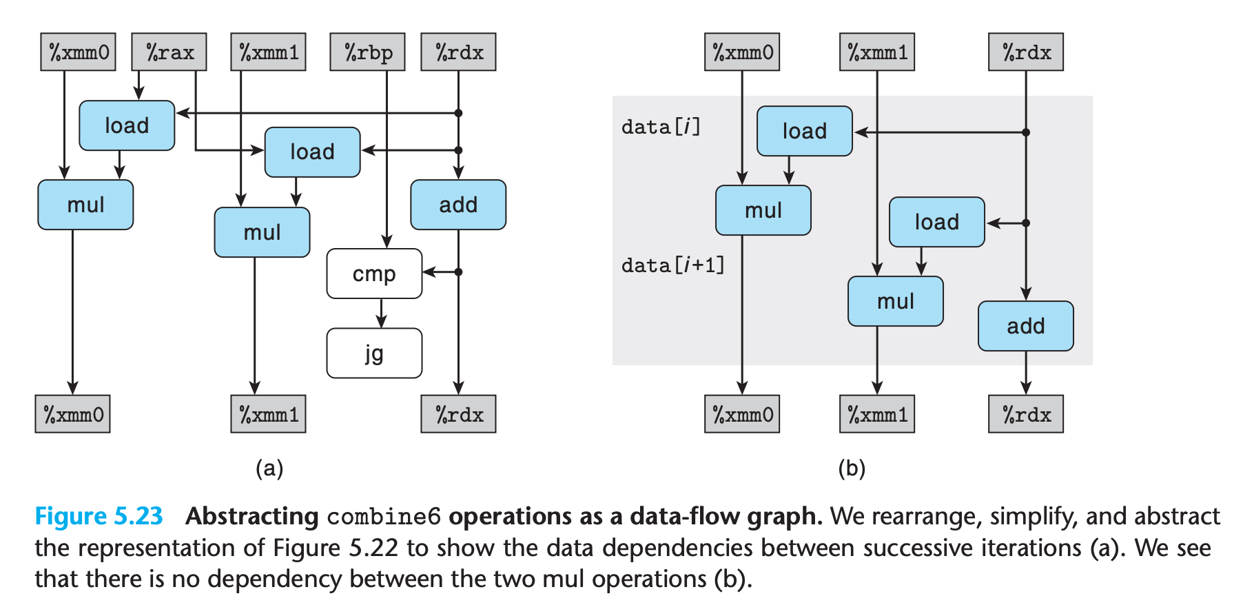
We now explore another way to break the sequential dependencies and thereby improve performance beyond the latency bound
1 | acc = (acc OP data[i]) OP data[i+1]; |
You may wondering how such a subtle change can make performance improvement since it still need 2 arithmetic which cannot be run in parallel.
The data flow graph give a clear view
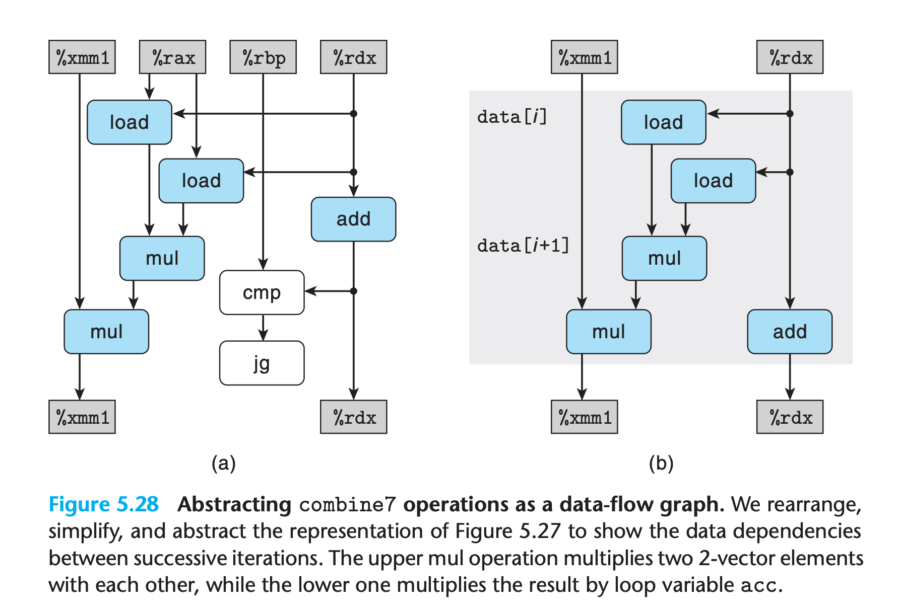
- the operation
data[i] OP data[i+1]do not need to wait for the previous iteration result, it can be done independently - As with the templates for combine5 and combine7, we have two load and two mul operations, but only one of the mul operations forms a data-dependency chain between loop registers
- we only have
n/2operations along the critical path.
We can see that this transformation yields performance results similar to what is achieved by maintaining k separate accumulators with k × k unrolling
In performing the reassociation transformation, we once again change the order in which the vector elements will be combined together.
The assessment is just like the one in k × k unrolling.
Practice Problem 5.8
Consider the following function for computing the product of an array of n double precision numbers. We have unrolled the loop by a factor of 3.
2
3
4
5
6
7
8
9
10
11
12
13
14
15
{
long i;
double x, y, z;
double r = 1;
for (i = 0; i < n-2; i+= 3) {
x = a[i];
y = a[i+1];
z = a[i+2];
r = r * x * y * z; /* Product computation */
}
for (; i < n; i++)
r *= a[i];
return r;
}For the line labeled “Product computation,” we can use parentheses to create five different associations of the computation, as follows:
2
3
4
5
r = (r * (x * y)) * z; /* A2 */
r = r * ((x * y) * z); /* A3 */
r = r * (x * (y * z)); /* A4 */
r = (r * x) * (y * z); /* A5 */Assume we run these functions on a machine where floating-point multiplication has a latency of 5 clock cycles. Determine the lower bound on the CPE set by the data dependencies of the multiplication. (Hint: It helps to draw a data-flow representation of how r is computed on every iteration.)
My solution : (:x: for A3 and A4)
1 | /* A1 */ |
Solution on the book :
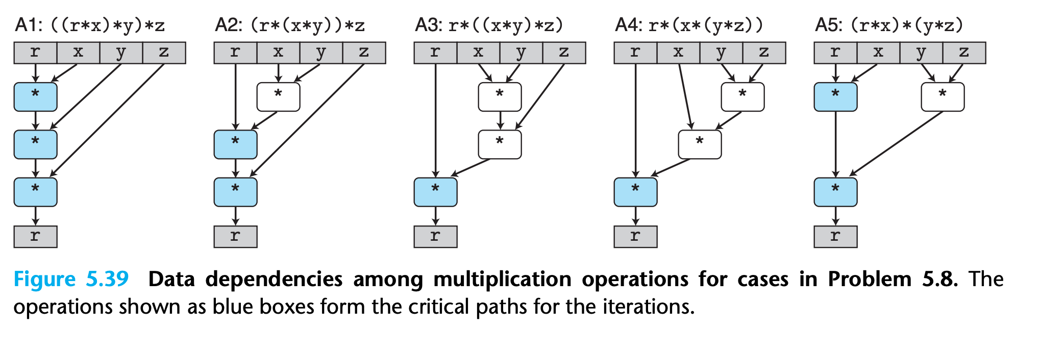
Note that only operation with a data dependency can form a critical path !!!
Hence the critical path of A3 and A4 is still the left side.
Intel introduced the SSE instructions in 1999, where SSE is the acronym for “streaming SIMD extensions”
The SSE capability has gone through multiple generations, with more recent versions being named advanced vector extensions, or AVX.
AVX instructions can perform vector operations on registers(
%ymm0 ~ %ymm15), such as adding or multiplying eight or four sets of values in parallel
gcc supports extensions to the C language that let programmers express a program in terms of vector operations that can be compiled into the vector instructions of AVX
This coding style is preferable to writing code directly in assembly language.
This will also faciliate improve our performance.
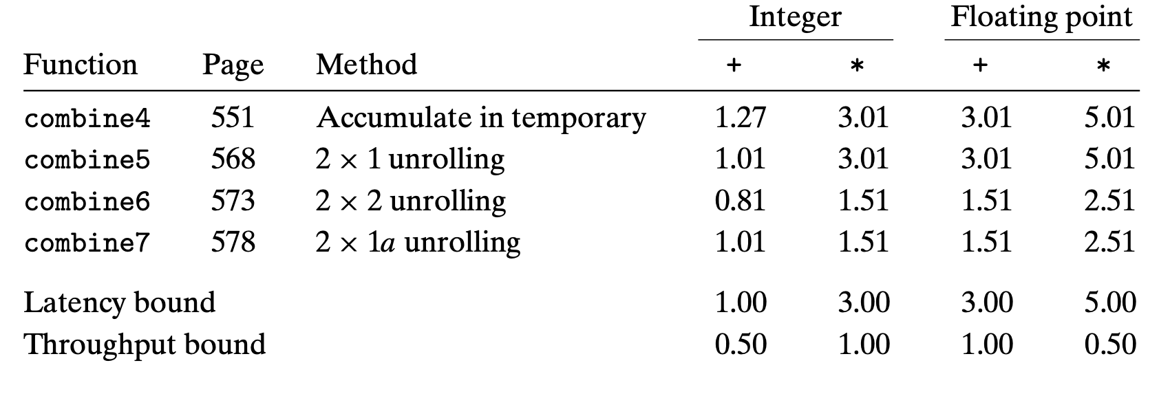
Using a combination of gcc instructions, loop unrolling, and multiple accumulators, we are able to achieve the following performance for our combining functions
5.10 Summary of Results for Optimizing Combining Code
Our example demonstrates that modern processors have considerable amounts of computing power, but we may need to coax this power out of them by writing our programs in very stylized ways.
5.11 Some Limiting Factors
In this section, we will consider some other factors that limit the performance of programs on actual machines.
5.11.1 Register Spilling
If a program has a degree of parallelism P that exceeds the number of available registers, then the compiler will resort to spilling, storing some of the temporary values in memory, typically by allocating space on the run-time stack.
For example
1 | #acc0 *= data[i] |
When register spilling happens the performance of our program may get worse rather than better.
5.11.2 Branch Prediction and Misprediction Penalties
A conditional branch can incur a significant misprediction penalty when the branch prediction logic does not correctly anticipate whether or not a branch will be taken
In a processor that employs speculative execution, the processor begins executing the instructions at the predicted branch target.
It does this in a way that avoids modifying any actual register or memory locations until the actual outcome has been determined.
- If the predication is correct, the results will be “committed”
- If the predication is wrong, the results will be discard
The misprediction penalty is incurred in doing this, because the instruction pipeline must be refilled before useful results are generated.
So how can we avoid this ?
There is no simple answer to this question, but the following general principles apply.
Do Not Be Overly Concerned about Predictable Branches
- the branch prediction logic found in modern processors is very good at discerning regular patterns and long-term trends for the different branch instructions(with almost 90% accuracy)
Write Code Suitable for Implementation with Conditional Moves
This cannot be controlled directly by the C programmer, but some ways of expressing conditional behavior can be more directly translated into conditional moves than others.
We have found that gcc is able to generate conditional moves for code written in a more “functional” style, where we use conditional operations to compute values and then update the program state with these values(use
? :!!!), as opposed to a more “imperative” style, where we use conditionals to selectively update program state.For example
1
2
3
4
5
6
7
8
9
10
11
12
13
14
15
16
17
18
19
20
21
22/* Rearrange two vectors so that for each i, b[i] >= a[i] */
void minmax1(long a[], long b[], long n) {
long i;
for (i = 0; i < n; i++) {
if (a[i] > b[i]) {
long t = a[i];
a[i] = b[i];
b[i] = t;
}
}
}
/* Rearrange two vectors so that for each i, b[i] >= a[i] */
void minmax2(long a[], long b[], long n) {
long i;
for (i = 0; i < n; i++) {
long min = a[i] < b[i] ? a[i] : b[i];
long max = a[i] < b[i] ? b[i] : a[i];
a[i] = min;
b[i] = max;
}
}Examing the assembly code or even embed assembly code directly is always the most realiable way.
5.12 Understanding Memory Performance
All modern processors contain one or more cache memories to provide fast access to small amounts of memory
5.12.1 Load Performance
In most of the cases, memory won’t be a bottleneck, whereas sometimes data dependency happens in loading will be a optimization blocker.
For example count the length of a linked list
1 | typedef struct node { |
1 | .L3 |
5.12.2 Store Performance
A series of store operations cannot create a data dependency since they don’t change register value in their very nature
Only a load operation is affected by the result of a store operation, since only a load can read back the memory value that has been written by the store.
For example
1 | /* Set elements of array to 0 */ |
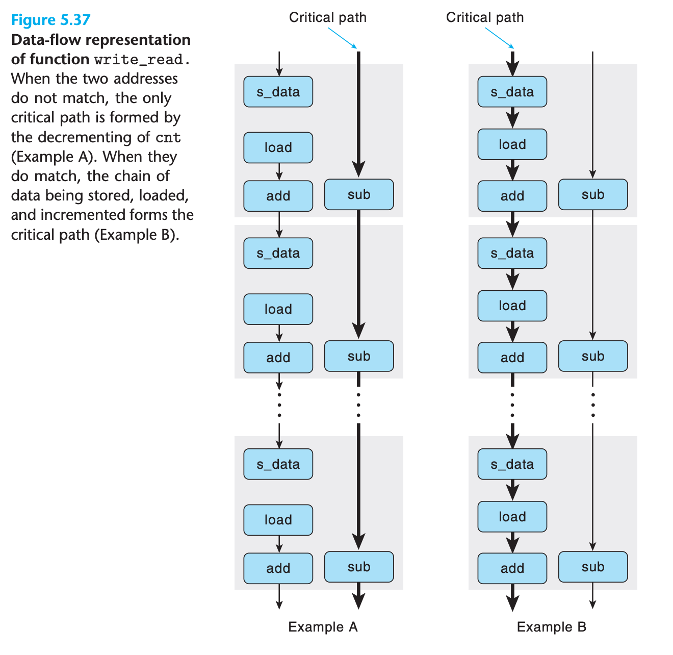
However combine load and store together we can have complex dependency
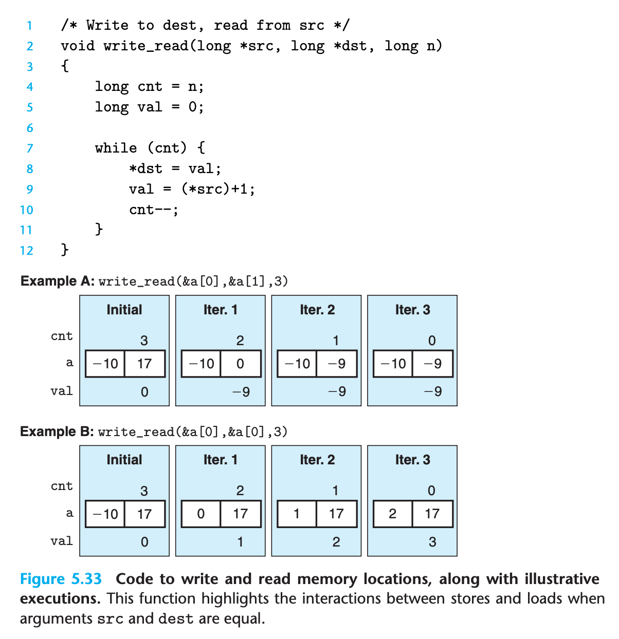
- Measuring example A over a larger number of iterations gives a CPE of 1.3 since the read operation is not affected by write operation
- Example B has a CPE of 7.3, the write/read dependency causes a slowdown in the processing of around 6 clock cycles.(it must wait for data to be written into the memory and then read it out)
Practice Problem 5.10
As another example of code with potential load-store interactions, consider the following function to copy the contents of one array to another:
2
3
4
5
6
{
long i;
for (i = 0; i < n; i++)
dest[i] = src[i];
}Suppose
ais an array of length 1,000 initialized so that each elementa[i]equalsi.A. What would be the effect of the call
copy_array(a+1,a,999)?B. What would be the effect of the call
copy_array(a,a+1,999)?C. Our performance measurements indicate that the call of part A has a CPE of 1.2 (which drops to 1.0 when the loop is unrolled by a factor of 4), while the call of part B has a CPE of 5.0. To what factor do you attribute this performance difference?
D. What performance would you expect for the call
copy_array(a,a,999)?
My solution : :white_check_mark:
A: move a[1~999] to a[0~998]
B: move a[0~998] to a[1~999]
C: because A doesn’t form data dependency, the value to be read is not connected with the previous operation while B is exactly the opposite
D: same performance with A
5.13 Life in the Real World: Performance Improvement Techniques
We have described a number of basic strategies for optimizing program performance
- High-level design
- Choose appropriate algorithms and data structures for the problem at hand
- Basic coding principles(use local variables)
- Eliminate excessive function calls
- Eliminate unnecessary memory references
- Low-level optimizations
- Unroll loops to reduce overhead and to enable further optimizations.
- Find ways to increase instruction-level parallelism by techniques such as multiple accumulators and reassociation
- Rewrite conditional operations in a functional style to enable compilation via conditional data transfers.(use
cmov)
It is very easy to make mistakes when introducing new variables, changing loop bounds, and making the code more complex overall, please test them extensively!
5.14 Identifying and Eliminating Performance Bottlenecks
When working with large programs, even knowing where to focus our optimization efforts can be difficult.
5.14.1 Program Profiling
Program profiling involves running a version of a program in which instrumentation code has been incorporated to determine how much time the different parts of the program require
Unix systems provide the profiling program gprof
- It determines how much CPU time was spent for each of the functions in the program
- It computes a count of how many times each function gets called, categorized by which function performs the call.
Steps to use gprof
- The program must be compiled and linked for profiling.
1 | $ gcc -Og -pg prog.c -o prog |
- Run the program as usual
1 | $ ./prog |
It will generate a gmon.out file
gprofis invoked to analyze the data
1 | $ gprof prog |
Some properties of gprof are worth noting
- The timing is not very precise due to OS interruption mechanism
- . The calling information is quite reliable, assuming no inline substitutions have been performed.
- By default, the timings for library functions are not shown