Following the Sympy tutorial
This tutorial assumes a decent mathematical background.
What is Symbolic Computation?
the mathematical objects are represented exactly, not approximately, and mathematical expressions with unevaluated variables are left in symbolic form.
1 | import sympy as s |
Unlike many symbolic manipulation systems, variables in SymPy must be defined before they are used
Create symbols
1 | x,y=s.symbols("x y") |
Use symbols
symbolstakes a string of variable names separated by spaces or commas, and creates Symbols out of them.
1 | expr = x + 2*y |
most simplifications are not performed automatically.
Both forms are useful in different circumstances.
In SymPy, there are functions to go from one form to the other
Simplification
1 | simplify = s.expand |
The Power of Symbolic Computation
The real power of a symbolic computation system such as SymPy is the ability to do all sorts of computations symbolically. SymPy can simplify expressions, compute derivatives, integrals, and limits, solve equations, work with matrices, and much, much more, and do it all symbolically. It includes modules for plotting, printing (like 2D pretty printed output of math formulas, or LATEX), code generation, physics, statistics, combinatorics, number theory, geometry, logic, and more.
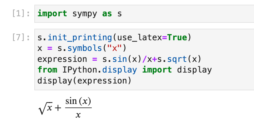
Prettify the output
1 | help(s.init_printing) |
1 | init_printing(pretty_print=True) # default argument |
1 | s.init_printing(use_unicode=True) |
1 | s.init_printing(use_latex='mathjax') |
Get the latex expression
1 | s.latex(s.diff(s.sin(x)*s.exp(x) , x)) |
Derivative
1 | s.diff(expression , x) |
Integral
1 | s.integrate(expression , x) |
Limit
1 | s.limit(expression,x,to_what) |
Normal equation
1 | s.solve(expression , x) # expression = 0 |
Differential equation
1 | y = s.Function("y") |
Gotcha
To begin, we should make something about SymPy clear.
SymPy is nothing more than a Python library, like
NumPy,Django, or even modules in the Python standard librarysysorre.What this means is that SymPy does not add anything to the Python language.
Gotcha1
Symbols can have names longer than one character if we want.
1 | crazy = sympy.symbols("unrelated") |
==So it’s a good idea to let symbol names and Python variable names coincide !!==
Update value in a expression
- Evaluating an expression at a point. For example, if our expression is
cos(x) + 1and we want to evaluate it at the pointx = 0, so that we getcos(0) + 1, which is 2. - Replacing a subexpression with another subexpression.
- To perform multiple substitutions at once, pass a list of
(old, new)pairs tosubs.
1 | expr = x + y(x) |
1 | expr |
There are two important things to note about subs. First, it returns a new expression. SymPy objects are immutable. That means that subs does not modify it in-place.
==In fact, since SymPy expressions are immutable, no function will change them in-place. All functions will return new expressions !==
Gotcha2
SymPy does not extend Python syntax is that = does not represent equality in SymPy.
There is a separate object, called Eq, which can be used to create symbolic equalities
1 | s.Eq(y(x) , s.exp(x)) |
Gotcha3
Do not use == to test if two expressions are equal, use a.equals(b) instead
1 | a = cos(x)**2 - sin(x)**2 |
Gotcha4
Combination of different types
Whenever you combine a SymPy object and a SymPy object, or a SymPy object and a Python object, you get a SymPy object, but whenever you combine two Python objects, SymPy never comes into play, and so you get a Python object.
SymPy Features
Converting Strings to SymPy Expressions
The sympify function (that’s sympify, not to be confused with simplify) can be used to convert strings into SymPy expressions.
Warning :
sympifyuseseval. Don’t use it on unsanitized input.
1 | new = sympify('z**4 + z**2 + z') |
Evaluate an expression
To evaluate a numerical expression into a floating point number, use evalf.
SymPy can evaluate floating point expressions to arbitrary precision. By default, 15 digits of precision are used, but you can pass any number as the argument to evalf.
1 | expr.subs(y , x**2) |
it is more efficient and numerically stable to pass the substitution to evalf using the subs flag, which takes a dictionary of Symbol: point pairs.
1 | new.evalf( 3, subs={z:5}) |
Sometimes there are roundoff errors smaller than the desired precision that remain after an expression is evaluated. Such numbers can be removed at the user’s discretion by setting the chop flag to True.
1 | one = cos(1)**2 + sin(1)**2 |
if you wanted to evaluate an expression at a thousand points, using SymPy would be far slower than it needs to be, especially if you only care about machine precision. Instead, you should use libraries like NumPy and SciPy.
Lambdify
lambdify acts like a lambda function, except it converts the SymPy names to the names of the given numerical library, usually NumPy.
1 | import numpy |
Warning :
lambdifyuseseval. Don’t use it on unsanitized input.
Printing
There are several printers available in SymPy. The most common ones are
- str
- srepr
- ASCII pretty printer
- Unicode pretty printer
- LaTeX
- MathML
- Dot
In order to see latex output, you should in an GUI Python console, for example, JupyterNoteBook
Simplification
SymPy has dozens of functions to perform various kinds of simplification. There is also one general function called simplify() that attempts to apply all of these functions in an intelligent way to arrive at the simplest form of an expression.
the gamma function
$$
\Gamma(n) = (n-1)!
$$
1 | simplify(gamma(x)/gamma(x-1)) |
simplify()is best when used interactively, when you just want to whittle down an expression to a simpler form. You may then choose to apply specific functions once you see whatsimplify()returns, to get a more precise result. It is also useful when you have no idea what form an expression will take, and you need a catchall function to simplify it
Polynomial/Rational Function Simplification
Given a polynomial, expand() will put it into a canonical form of a sum of monomials.
1 | expand( (x-2)**2 + (x+sqrt(2))**2) |
factor() takes a polynomial and factors it into irreducible factors over the rational numbers. For polynomials, factor() is the opposite of expand().
1 | factor( x**2 - 2*x + 1) |
collect() collects common powers of a term in an expression.
1 | collect( 2*x**2 + 4*x**4 + 16*x**16 + 7*x**7 , x) |
expr.coeff(x, n) gives the coefficient of x**n in expr
1 | collect( 2*x**2 + 4*x**4 + 16*x**16 + 7*x**7 , x).coeff(x,16) |
cancel() will take any rational function and put it into the standard canonical form
1 | cancel( (x-2)**3 / (x-2) ) |
apart() performs a partial fraction decomposition on a rational function
Trigonometric Simplification
Power
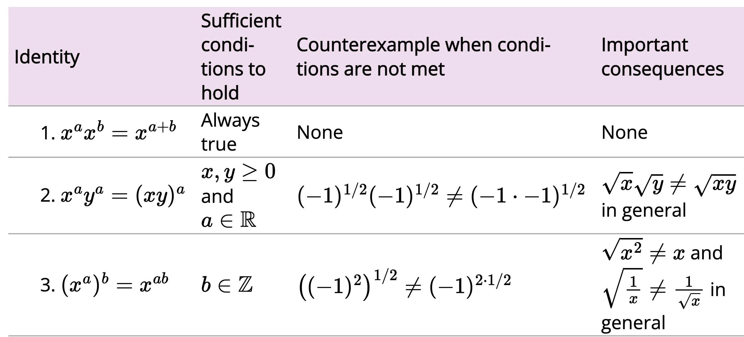
This is important to remember, because by default, SymPy will not perform simplifications if they are not true in general.
1 | # so we can specify type of number when we defining they |
Exponentials and logarithms
Logarithms have similar issues as powers.
Special Functions
SymPy implements dozens of special functions, ranging from functions in combinatorics to mathematical physics.
factorial(n)binomial(n, k)- ….
Rewrite
To rewrite an expression in terms of a function,useexpr.rewrite(function)
1 | gamma(x).rewrite(factorial) |
Piecewise Functions
1 | formula = Piecewise( (x**2, x>2), (1+x, x<=2) ) |
Combine Functions
1 | f |
$$
f = \begin{cases} \ln{\sqrt{x}} , & x \ge 1\
2x-1 , & x<1
\end{cases}
$$
$$
ff = f(f(x))
$$
Calculus
Tips
Do differential n times
1 | def d(f,n): |
Taylor expansion
Taylor expansion with Peano Reminder at x0
1 | x = s.symbols('x') |
1 | # For abstract f=f(x) |