Vector Space

“Closed” on addition and scale operation

So every vector space must have the origin point, $(0,0,…,0)$

Example

$R^2$ = all 2-D vectors = the whole plane

Sub Vector Space

only part of the whole vector space, and still satisfy the rules

Example : all subspace of $R^3$

• all of $R^3$

• any line through the origin

• any plane through the origin

• the original point only

Conclusion

columns of matrix can form a space including all the linear combinations of columns

Property

if $V$ and $W$ are both subspace of $R^n$

• $V \cap W$ is still a subspace

• $V \cup W$ is not a subspace

(Think $R^3$ as an example)

Column Space

Given a matrix, the linear combination of columns of it might form a (sub)space

Example

$$
\begin{bmatrix}
1&3\
2&4
\end{bmatrix}
$$

$\begin{bmatrix} 1\2 \end{bmatrix}$ and $\begin{bmatrix} 3\4 \end{bmatrix}$ forms a $R^2$ space

$$
\begin{bmatrix}
1&8\
2&5\
6&7
\end{bmatrix}
$$

Forms a subspace in $R^3$

Connection with equations

$$
A\vec{x}=B
$$

We can view A’s columns as vectors, their linear combination form a column space. B is all dots in that space.

Example

$$
A\vec{x} = \begin{bmatrix} 1 & 1 & 2 \
2 & 1 & 3 \
3 & 1 & 4 \
4 & 1 & 5
\end{bmatrix}
\begin{bmatrix}
x_1 \
x_2 \
x_3 \
\end{bmatrix}
= \begin{bmatrix}
b_1 \ b_2 \ b_3 \ b_4 \end{bmatrix} =B
$$

Which B allow the system to be solved ?

When B is in the column space of A!!!

Null space

if $B =0$, all possible $\vec{x}$ can form a space, we call it a null space(Actually show the “dependencies” in A’s columns)

Example

$$
A\vec{x} = \begin{bmatrix} 1 & 1 & 2 \
2 & 1 & 3 \
3 & 1 & 4 \
4 & 1 & 5
\end{bmatrix}
\begin{bmatrix}
x_1 \
x_2 \
x_3 \
\end{bmatrix}
= \begin{bmatrix}
0 \ 0 \ 0 \ 0 \end{bmatrix} =B
$$

We can see for any $A$, $\vec{x} = 0$ must be a solution

For this particular $A$, we inspect that column 3 is a linear combination of column 1 and 2, so it can be dropped, so we have the solution

Null space = $C \begin{bmatrix} 1 \ 1 \ -1 \ \end{bmatrix}$, C can be any constant , including 0

Algorithm for solving $A\vec{x}=0$

Elimination + Specify free + Linear Combination

Example

$$
A = \begin{bmatrix}
1 & 2 & 2 & 2\
2 & 4 & 6 & 8\
3 & 6 & 8 & 10
\end{bmatrix}
$$

What is the null space of $A$ ?

Step 1 : Gaussian Elimination

$$
E_{21}A = \begin{bmatrix}
1 & 2 & 2 & 2\
0 & 0 & 2& 4\
3 & 6 & 8 & 10
\end{bmatrix}
$$

$$
E_{31}(E_{21}A) = \begin{bmatrix}
1 & 2 & 2 & 2\
0 & 0 & 2& 4\
0 & 0 & 2 & 4
\end{bmatrix}
$$

$$
E_{33}E_{31}E_{21}A=\begin{bmatrix}
1 & 2 & 2 & 2\
0 & 0 & 2& 4\
0 & 0 & 0 & 0
\end{bmatrix} =
\Bigg[
\begin{array}{}

\begin{array}{cc}
\textcircled{1} & 2 \\hline
0 & 0 \
0 & 0
\end{array}

\begin{array}{cc}
2 & 2 \
\textcircled{2} & 4 \\hline
0 & 0
\end{array}
\end{array}
\Bigg]
$$

We call this an echelon matrix, the circled 1 and 2 are called pivots

The number of pivots is called rank, in this example is $2$

From my own perspective, the rank means the number of “unique” vectors/rows, non-unique ones can be obtained by linear combination of unique ones, so they do not contribute new stuff, they can in turn be dropped, as a result they are cancelled out in the elimination

rank == len(pivot_variables)
freenom == len(len(columns) - rank) == len(free_variables)

Columns with pivot are called pivot column, those do not have pivots are called free columns

Step 2 : Assign arbitrary value for free variables

We can see that $x_1$ and $x_3$ are pivots, $x_2$ and $x_4$ are free variables

$$
\text{let}
\begin{cases}
x_2 = 1\
x_4 = 0
\end{cases}
$$

$$
\text{we see a special solution is :}
\begin{bmatrix}
x_1 \
x_2 \
x_3 \
x_4
\end{bmatrix}
=
\begin{bmatrix}
-2 \
1 \
0 \
0
\end{bmatrix}
$$

$$
\text{let}
\begin{cases}
x_2 = 0\
x_4 = 1
\end{cases}
$$

$$
\text{we see another special solution is :}
\begin{bmatrix}
x_1 \
x_2 \
x_3 \
x_4
\end{bmatrix}
=
\begin{bmatrix}
2 \
0 \
-2 \
1
\end{bmatrix}
$$

Step 3 : Linear combination

As we known that a linear combination of independent vectors will form a vector space, so

$$
\text{the space/ all solutions} = C_1\begin{bmatrix}
-2 \
1 \
0 \
0
\end{bmatrix} + C_2\begin{bmatrix}
2 \
0 \
-2 \
1
\end{bmatrix},C_1,C_2 \in R
$$

---

Extra work : reduced row echelon matrix

Our echelon matrix can be reduced further more

Turn pivots into 1s

$$
\Bigg[
\begin{array}{}

\begin{array}{cc}
\textcircled{1} & 2 \\hline
0 & 0 \
0 & 0
\end{array}

\begin{array}{cc}
2 & 2 \
\textcircled{2} & 4 \\hline
0 & 0
\end{array}
\end{array}
\Bigg]
\stackrel{row2/=2}{=} \begin{bmatrix}
1 & 2 & 2 & 2\
0 & 0 & 1& 2\
0 & 0 & 0 & 0
\end{bmatrix}
$$

Back substitution

$$
\begin{bmatrix}
1 & 2 & 2 & 2\
0 & 0 & 1& 2\
0 & 0 & 0 & 0
\end{bmatrix}
\stackrel{row1-=2row2}{=}
\begin{bmatrix}
1 & 2 & 0 & -2\
0 & 0 & 1& 2\
0 & 0 & 0 & 0
\end{bmatrix}
$$

Columns exchange

$$
\begin{bmatrix}
1 & 0 & 2 & -2\
0 & 1 & 0& 2\
0 & 0 & 0 & 0
\end{bmatrix}
=
\begin{bmatrix}
I & F\
0 & 0
\end{bmatrix}= R
$$

$R$ for reduced

$$
\text{Now our problem is :} R\vec{x}= \begin{bmatrix}
I & F\
0 & 0
\end{bmatrix} \vec{x} = 0
$$

$$
\therefore \vec{x} = \begin{bmatrix} -F \ I \end{bmatrix} = \begin{bmatrix} x_{pivot} \ x_{free} \end{bmatrix}
$$

(Since we can pick arbitrary free value, why not pick 1s and 0s for $x_{free}$)

$$
\because \begin{bmatrix}
I & F\
0 & 0
\end{bmatrix} \begin{bmatrix}
x_{pivot}\
x_{free}
\end{bmatrix} = 0
$$

$$
\therefore x_{pivot} = -Fx_{free}
$$

$$
\therefore \begin{bmatrix}
x_{1}\
x_{2}\
…\
x_k
\end{bmatrix} = -F
\begin{bmatrix}
x_{k+1}\
x_{k+2}\
…\
x_{n}
\end{bmatrix}
$$

>>> import sympy
>>> A = array([ [1,2,2,2] , [2,4,6,8] , [3,6,8,10] ])
>>> A
array([[ 1,  2,  2,  2],
       [ 2,  4,  6,  8],
       [ 3,  6,  8, 10]])
>>> sympy.Matrix( A ).rref()
(Matrix([
[1, 2, 0, -2],
[0, 0, 1,  2],
[0, 0, 0,  0]]), (0, 2))

---

Solving $A\vec{x} = B$

Why we have the pattern a particular solution + Null space = Complete solution ?

$$
\because \text{if we find a particular } \vec{x_p}, \text{that} A\vec{x_p}=B
$$

$$
\because A\vec{x_n} = 0
$$

$$
\therefore A(\vec{x_p} + \vec{x_n}) = B
$$

$$
\therefore \vec{x} = \vec{x_p} + \vec{x_n}
$$

Visualization of an example

Say if we have

$$
\vec{x} = \begin{bmatrix}
-2\
0 \
3 \
\end{bmatrix} + C_1\begin{bmatrix}
-2 \
1 \
0
\end{bmatrix} + C_2\begin{bmatrix}
2 \
0 \
-2 \
\end{bmatrix},C_1,C_2 \in R
$$

Then $\vec{x}$ is not a vector space(since it doesn’t go through origin point), it is an offset vector space(since $\vec{x_n}$ is a vector space)

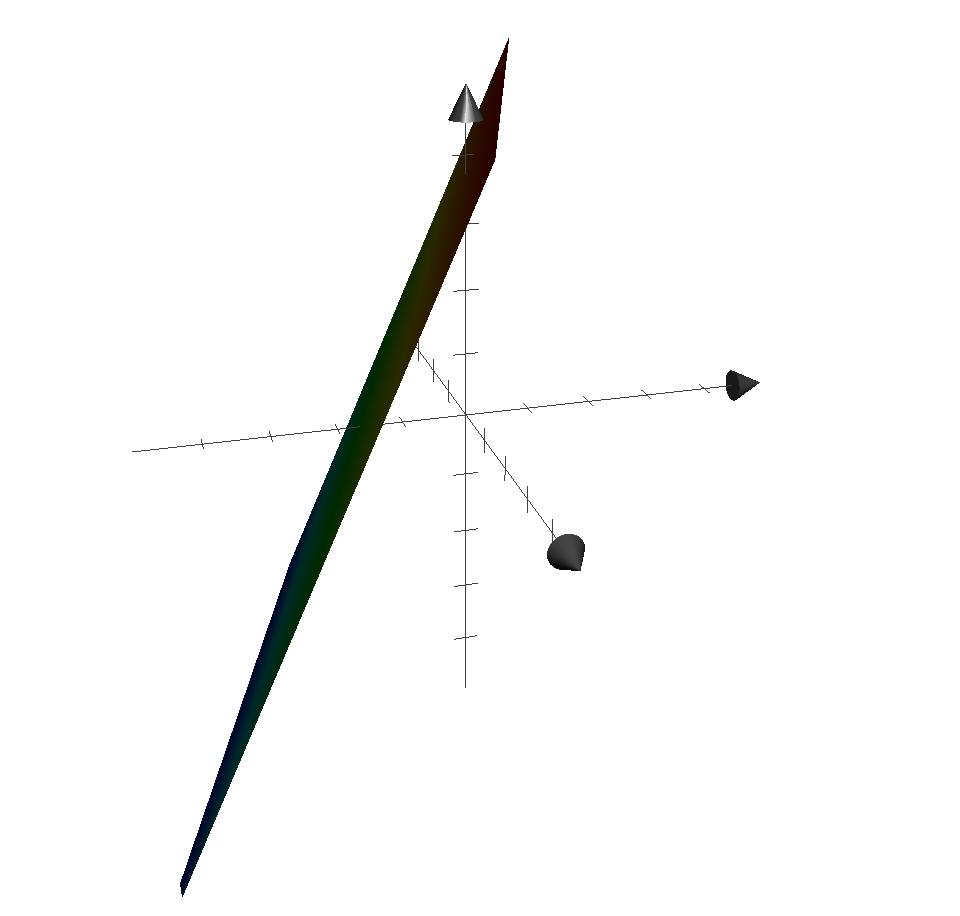
And the offset is given by the particular solution

Numbers of solution

For any matrix $m\times n$ we know that rank $r \le m , r \le n$

Full columns

$$
\text{if } r == n < m
$$

Then there will be only 1 solution in the null space, the zeros, so for $A\vec{x}=B$

$$
R = \begin{bmatrix}
I\
0
\end{bmatrix}
$$

$$
\text{number of solutions}=\begin{cases}
0,& \text{no particular solution}\
1 ,& \text{there is a particular solution}
\end{cases}
$$

Full rows

$$
\text{if } r == m < n
$$

number of unknown variables larger than number of constraints, we can solve the problem $A\vec{x}=B$ for any $B$

And there are $n-m$ free variables, so there is a null space

$$
R = \begin{bmatrix}
I&F
\end{bmatrix}
$$

$$
\text{There always be a complete solution}
$$

$$
\text{number of solutions}=\infty
$$

Full rank

$$
\text{if } r == m == n
$$

Then $A$ is square and will be invertible, $R= I$

Since it is full column, the null space is 0

Since it is full row, it can solve any $B$

$$
\text{There is 1 unique solution}
$$

Shrink rank

$$
\text{if } r < n \land r<m
$$

$$
R = \begin{bmatrix}
I & F\
0 & 0
\end{bmatrix}
$$

$$
\text{number of solutions}=\begin{cases}
0,& \text{we have 0 = non-0 for some }B\
\infty ,& \text{we can get a complete solution}
\end{cases}
$$

---

Independence

For vectors $\vec{x_1},\vec{x_2},…,\vec{x_n}$, if their linear combination do not gives $\vec{0}$(except $0\vec{x_1}+0\vec{x_2}+…+0\vec{x_n}$)

Firstly, according to the definition we can see that $\vec{0}$ has dependency with any other vector

$$
C\vec{0} + 0\vec{v} = \vec{0}
$$

Secondly, we can find that there is a connection with solving $A\vec{x}=0$

$$
\because \text{In full rows situation, the null space is not 0 }
$$

$$
\therefore \text{there are non-0 combination of A’s columns that gives } \vec{0}
$$

$$
\therefore \text{when m<n, there must be dependency}
$$

$$
\therefore \text{when r = n , the columns are independent, only 0 in null space}
$$

Example

If we have 3-vectors in 2-D space, there must be dependency, since $A$ is $2\times3$, $m<n$

Thirdly, we come with the basis of a vector space

For vectors $\vec{x_1},\vec{x_2},…,\vec{x_n}$, if their linear combination form a vector space and they are independent.

Then they are basis of this space.(Neither too few and nor too much)

And we inspect an important fact that

For $n$ vectors in $R^n$ space, if they are basis then the square matrix formed by them must be invertible

Since elimination will lead to $R=I$, that means $EA=R=I$, $E=A^{-1}$

Finally, we can see that all basis share the number of vectors, we call this number dimension of the space

Rank

rank(A) == len(pivot_columns) == dim(column_space_of_A)

len(columns) - rank(A) == len(free_columns) == dim(nullspace_of_A)

Example

$$
A = \begin{bmatrix}
1 & 0 & 2 & -2\
0 & 1 & 0& 2\
0 & 0 & 0 & 0
\end{bmatrix}
$$

rank(A) == 2 so the column space is a 2-dimension plane, and the null space is also 2-D

Four Fundamental Subspaces

• Column space $C(A)$

• Null space $N(A)$

• Row space $C(A^T)$

• Left null space of A $N(A^T)$

$$
\forall A = m \times n \text{ matrix }
$$

Space	Dimension	Basis
$C(A)$	$r$	Pivot Columns
$N(A)$	$n-r$	Free Columns
$C(A^T)$	$r$	Pivot Rows
$N(A^T)$	$m-r$	0-correspond rows in $E$

Example : basis of $N(A^T)$

We do Gaussian-Jordan to find elimination matrix $E$

$$
EA=R=\begin{bmatrix}I&F\
0 & 0
\end{bmatrix}
$$

So that we can see 0-correspond lines in $E$ tell that “This kind of combination of A’s rows gives a row of 0”

$$
\Big[A|I\Big] = \Bigg[
\begin{array}{cccc|ccc}
1 & 2 & 3 & 1 & 1&0&0\
1 & 1 & 2& 1 & 0&1&0\
1 & 2 & 3 & 1 & 0&0&1
\end{array}
\Bigg]
$$

$$
\Big[R|E\Big] = \Bigg[
\begin{array}{cccc|ccc}
1 & 0 & 1 & 1 & -1&2&0\
0 & 1 & 1& 0 & 1&-1&0\
0 & 0 & 0 & 0 & -1&0&1
\end{array}
\Bigg]
$$

$$
EA=R
$$

$$
\therefore -1 \times r1+0\times r2 + 1 \times r3 = 0
$$

$$
\therefore (-1,0,1) \text{is in left null space of A}
$$

$$
\text{A’s left null space} = C \begin{bmatrix} -1 \ 0 \ 1 \end{bmatrix}, C\in R
$$

---

In fact matrix can also be viewed as vectors, they can do addition and scalar multiplication

So we not only have vector space but also can have matrix space !

---

Example : Matrix Space

$$
A = \text{any } 3 \times 3 \text{ matrix}\
S = \text{any } 3 \times 3 \text{ symmetric matrix}\
U = \text{any } 3 \times 3 \text{ upper triangular matrix}
$$

If we take $A$ as a space formed by matrix(“the matrix space”),what is its dimension and basis ?

Since there are 9 different positions we can easily find that one of the basis is

$$
\begin{bmatrix}
1&0&0\
0&0&0\
0&0&0
\end{bmatrix},
\begin{bmatrix}
0&1&0\
0&0&0\
0&0&0
\end{bmatrix},…,
\begin{bmatrix}
0&0&0\
0&0&0\
0&0&1
\end{bmatrix},
$$

dim(A) == dim(3_3_matrix_space) == len(basis) == 9

And for upper triangular space and symmetric space we have

dim(U) == len(basis) == 6
dim(S) == len(basis) == 6

Let’s continue on to operate on the matrix spaces

$$
U \cap S = \text{matrixes both in } U,S,\text{the diagonal matrixes}
$$

$$
U \cup S = \text{matrixes either in } U \text{ or } S , \text{not a space!}
$$

$$
U + S = A
$$

We can surprisingly find that

dim(U + S) == 9
dim(U ∩ S) == 3
dim(U) == 6
dim(S) == 6

$$
dim(U+S)+dim(U\cap S) = dim(U)+dim(S)
$$

---

Example : linear differential equations

$$
y’’ +y = 0
$$

$$
r^2 + 0\cdot r+1 = 0
$$

$$
\alpha\pm\beta i = \frac{-b\pm\sqrt{4ac-b^2}}{2a} = \frac{\pm2i}{2}=\pm i
$$

$$
\therefore y = e^{\alpha x}(C_1 \sin(\beta x) + C_2 \cos(\beta x) = C_1 \sin x+C_2 cos x
$$

We can see $\sin x $ and $\cos x $ are “vectors” here, and they are one of the basis

We can get any solution by doing linear combination of them

So the dimension of this equation system is len(basis) == 2