Discrete Random Variable

Random “variables” are actually functions they are not variables!

It is a mapping or a function from possible outcomes in a sample space to a measurable space, often the real numbers.

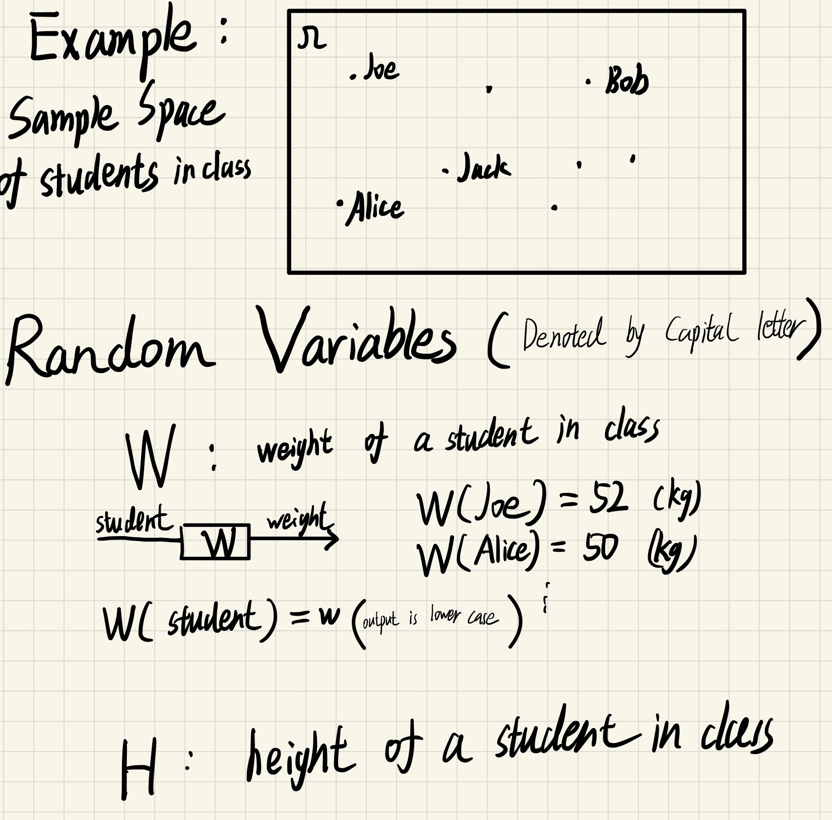
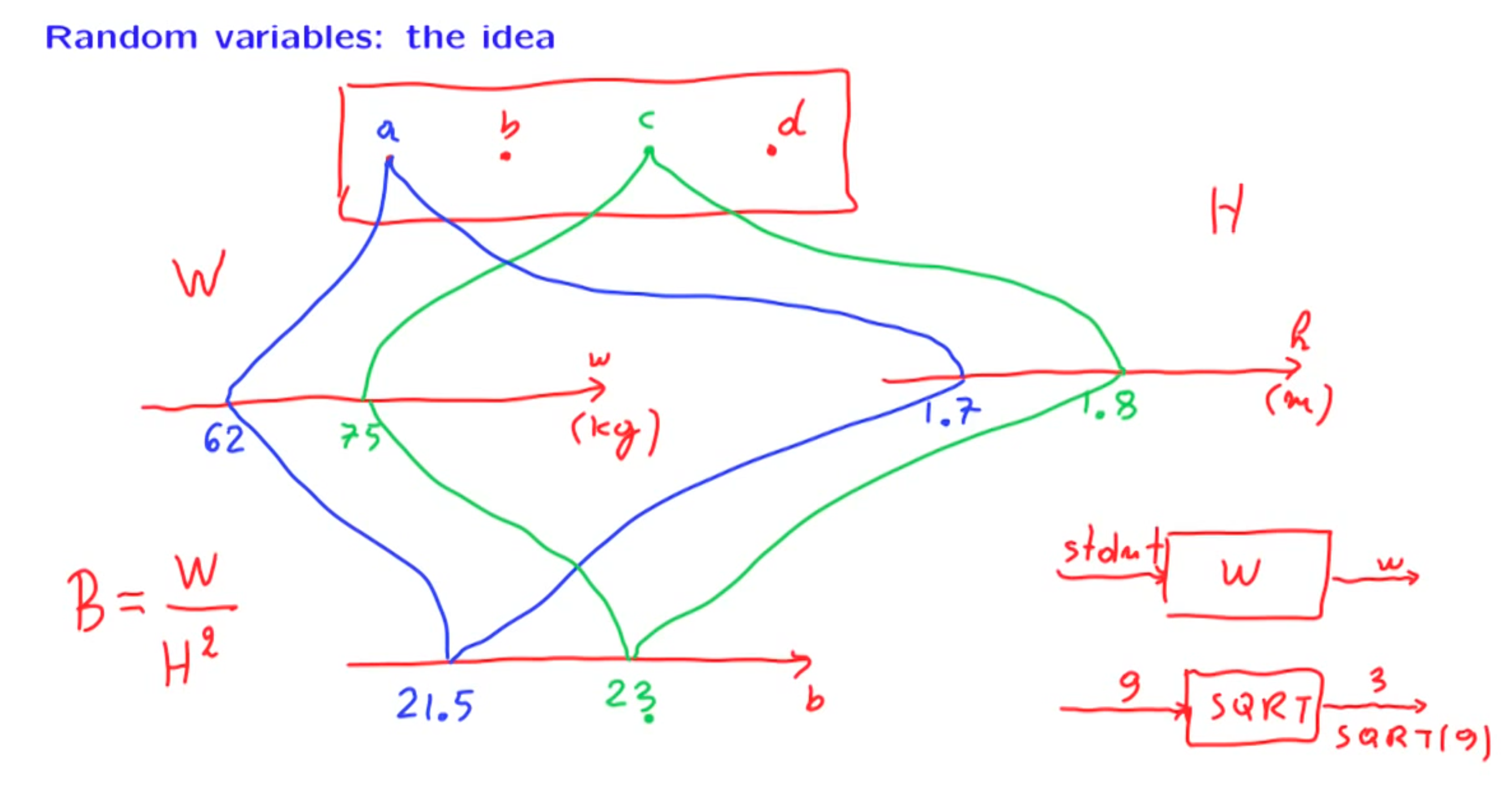
Random variables : associate a number to every possible outcome

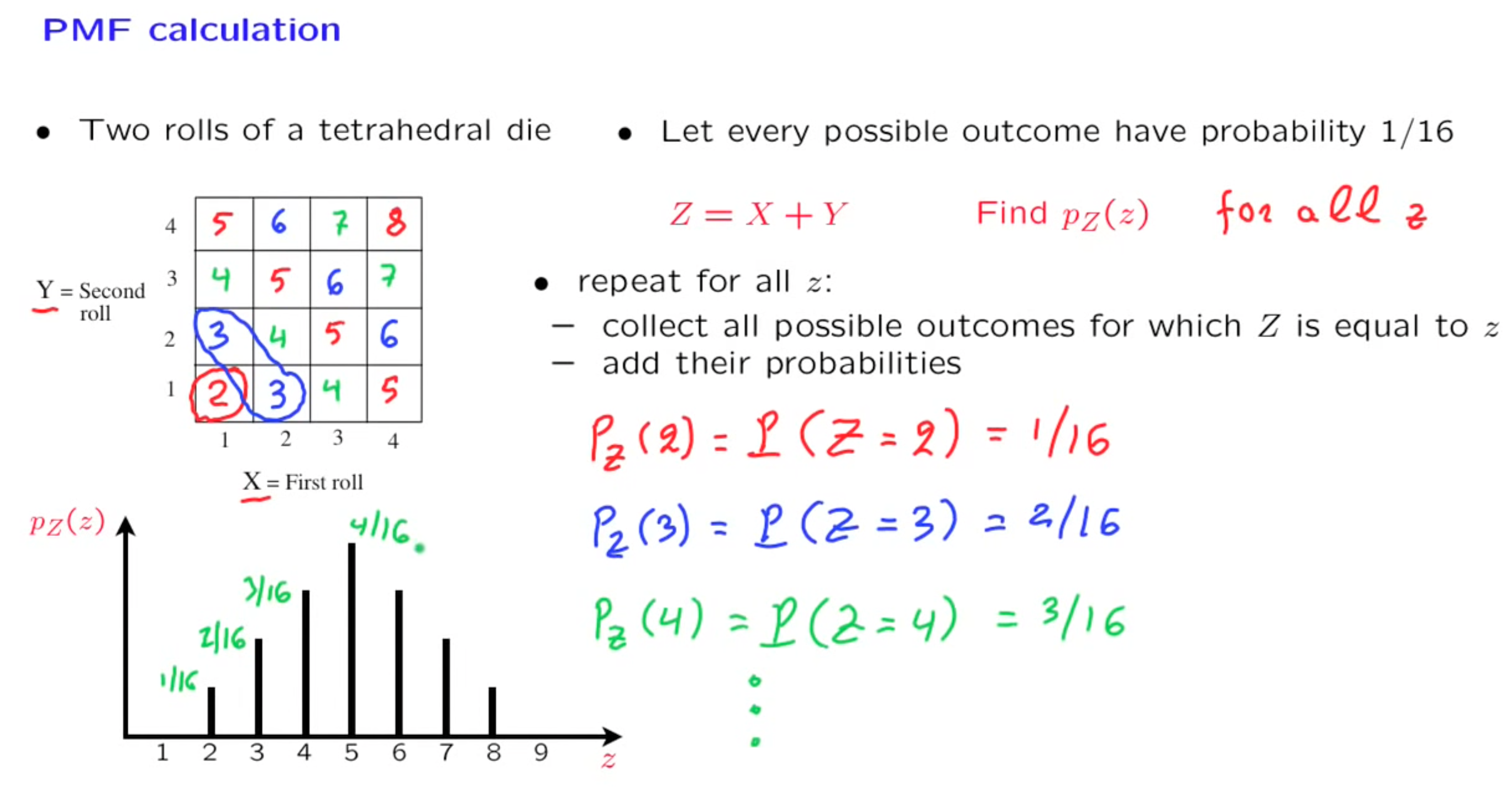
Probability mass function

The “probability law” or “probability distribution”

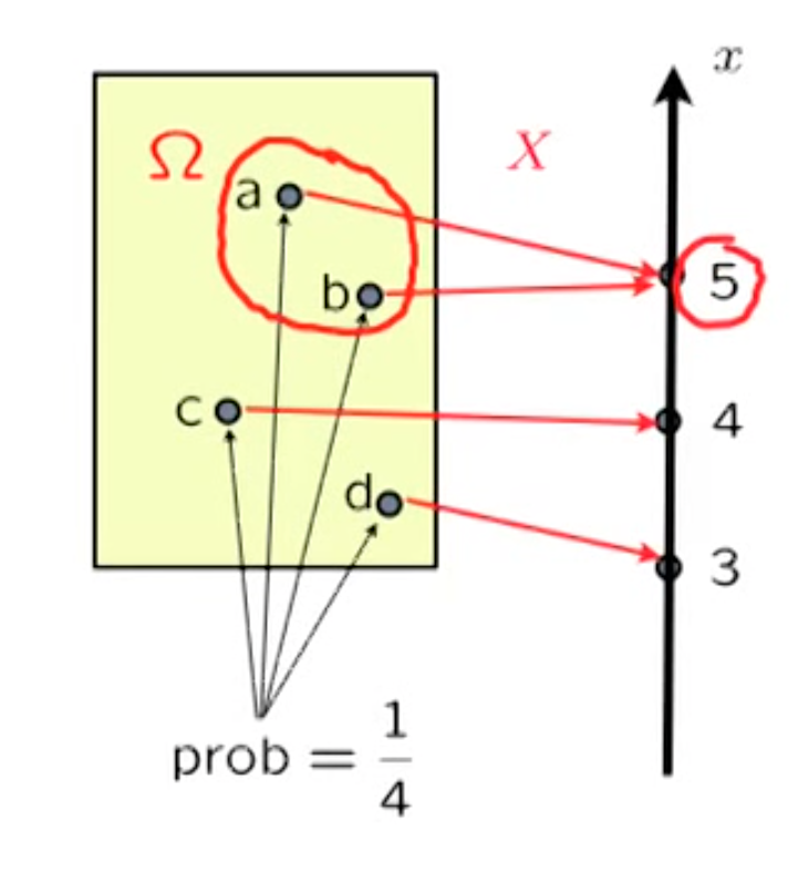
If we fix some $x$ , the $X = x$ is an event, we can have its probability

$$
P_X (x) = P(X=x)
$$

$$
\text{In this case :} P_X(5)=P(X=5) = \frac{1}{2}
$$

Then we can have a the probability mass function

$$
P_X(x)
$$

>>> Px(3)
1/4
>>> Px(4)
1/4
>>> Px(5)
1/2
>>> Px(1)
Traceback (most recent call last):
Exception: "Not in domain""

Property

$$
P_X(x) \ge 0
$$

$$
P_X(x_1)+P_X(x_2) + … + P_X(x_n) = 1
$$

Useful PMF

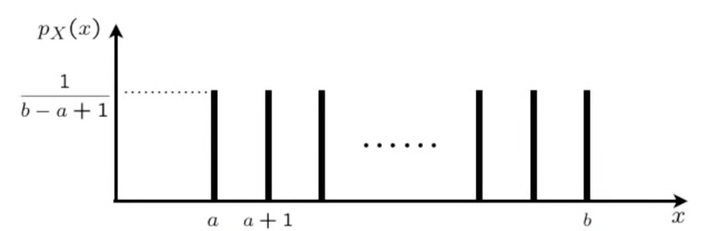
Uniform PMF

• experiment : random.randint(a,b)

• sample space : ${a,a+1,a+2,…,b-1,b}$

• Random Variable : $X : X(\text{result is x}) = x$

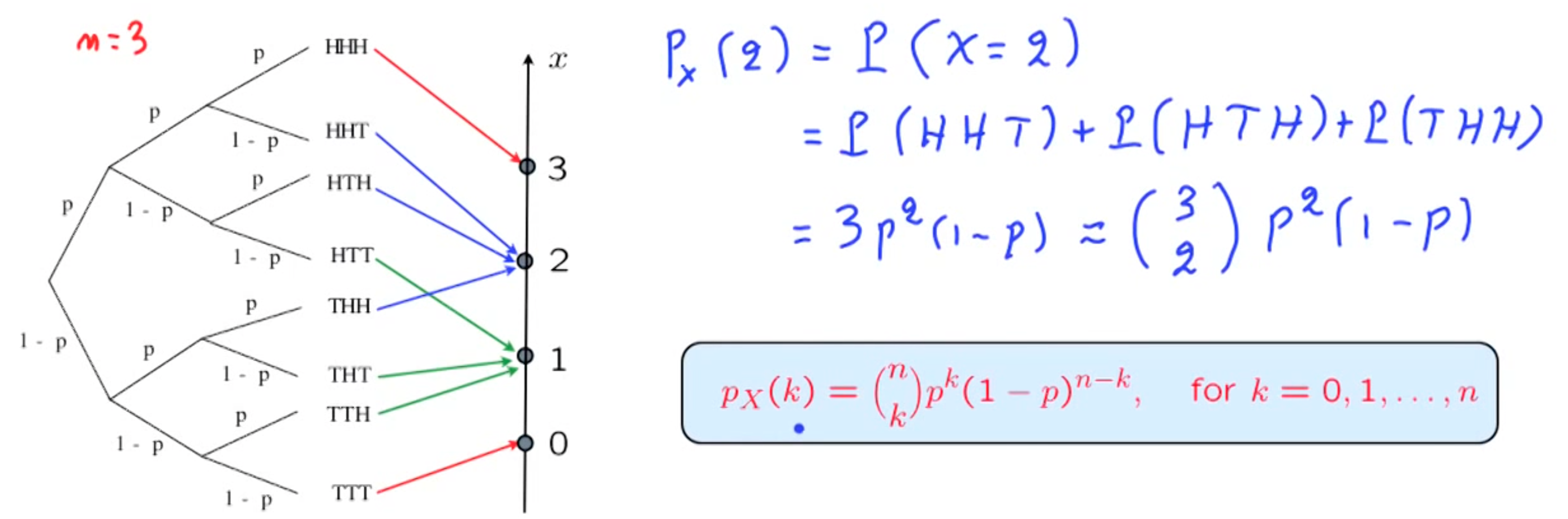
Binomial PMF

• experiment : toss a coin N times, with P(heads) = p

• sample space : ${H_1H_2…H_N , T_1H_2…H_N,….}$

• Random Variable : $X : X( \text{an outcome}) = \text{number of heads in this outcome}$

Geometry PMF

• experiment : keep tossing before heads appear

• sample space : ${H,TH,TTH,TTTH,….}$

• Random Variable : $X : X(\text{an sequence}) = \text{number of trials}$

$$
P_X(k) = P(X=k) = (1-p)^{k-1}p , k=1,2,3,…
$$

Expectation/Mean of Random Variable

.Average in large number of repetition of the experiment

For example, if you play a game with random variable like this

$$
x=\begin{cases}
1 , X(lose),P(lose) = \frac{2}{10}\
2 , X(equal),P(equal) = \frac{5}{10}\
4 , X(win) , P(win) = \frac{3}{10}
\end{cases}
$$

$$
\therefore P_X(x) = \begin{cases}
\frac{2}{10} , x = 1\
\frac{5}{10} , x = 2\
\frac{3}{10} , x = 4
\end{cases}
$$

When playing the game for 1000 times

I expect to get

$$
\text{Average Gain} = 1 \times 200 + 2 \times 500 + 4 \times 300
$$

$$
\therefore E[X] = \sum_{\text{all x}} P_X(x) \times x
$$

Obvious property

Expected value is the “balance” point for the PMF graph, the midpoint for symmetric graphs

remember that probability always add to 1

$$
a \le X\le b \implies a \le E[X] \le b
$$

$$
X(outcome) = C \Longrightarrow E[X] = C , \text{C is a constant}
$$

Expected Value rule, for $E[g(X)]$

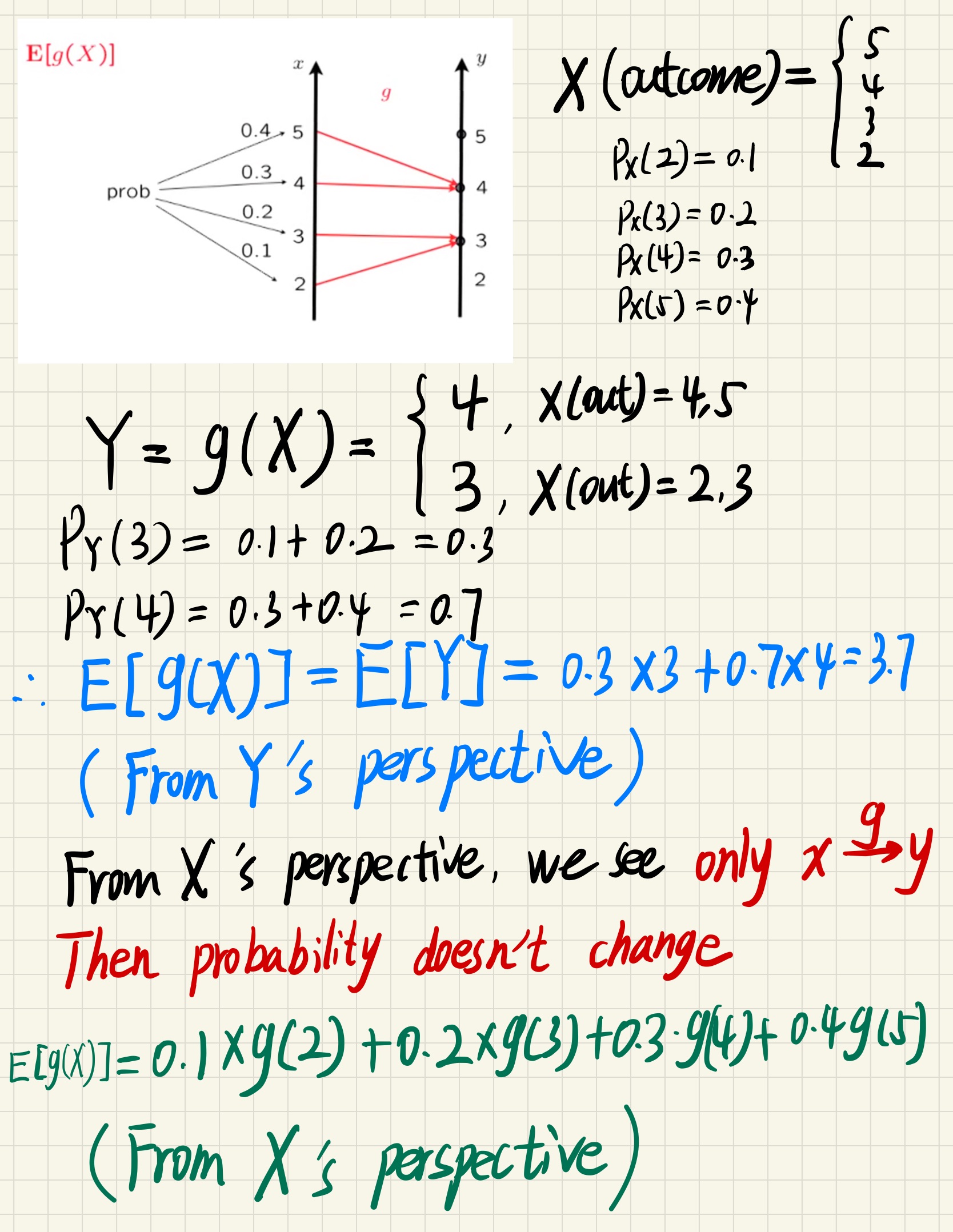
$$
\therefore E[g(X)] = \sum_{\text{for all} x} g(x) \times P_X(x)
$$

(Only value mapped, probability doesn’t change)

Linearity

proof

$$
E[aX+bY] = aE[X] + bE[Y]
$$

$$
E[aX+C] = aE[X]+C
$$

(If every ones’ salary doubled and raised 100, the average salary also doubled and raised 100)

---

---

---

Variance

Measure how the PMF spread.

Let $\mu = E[X]$

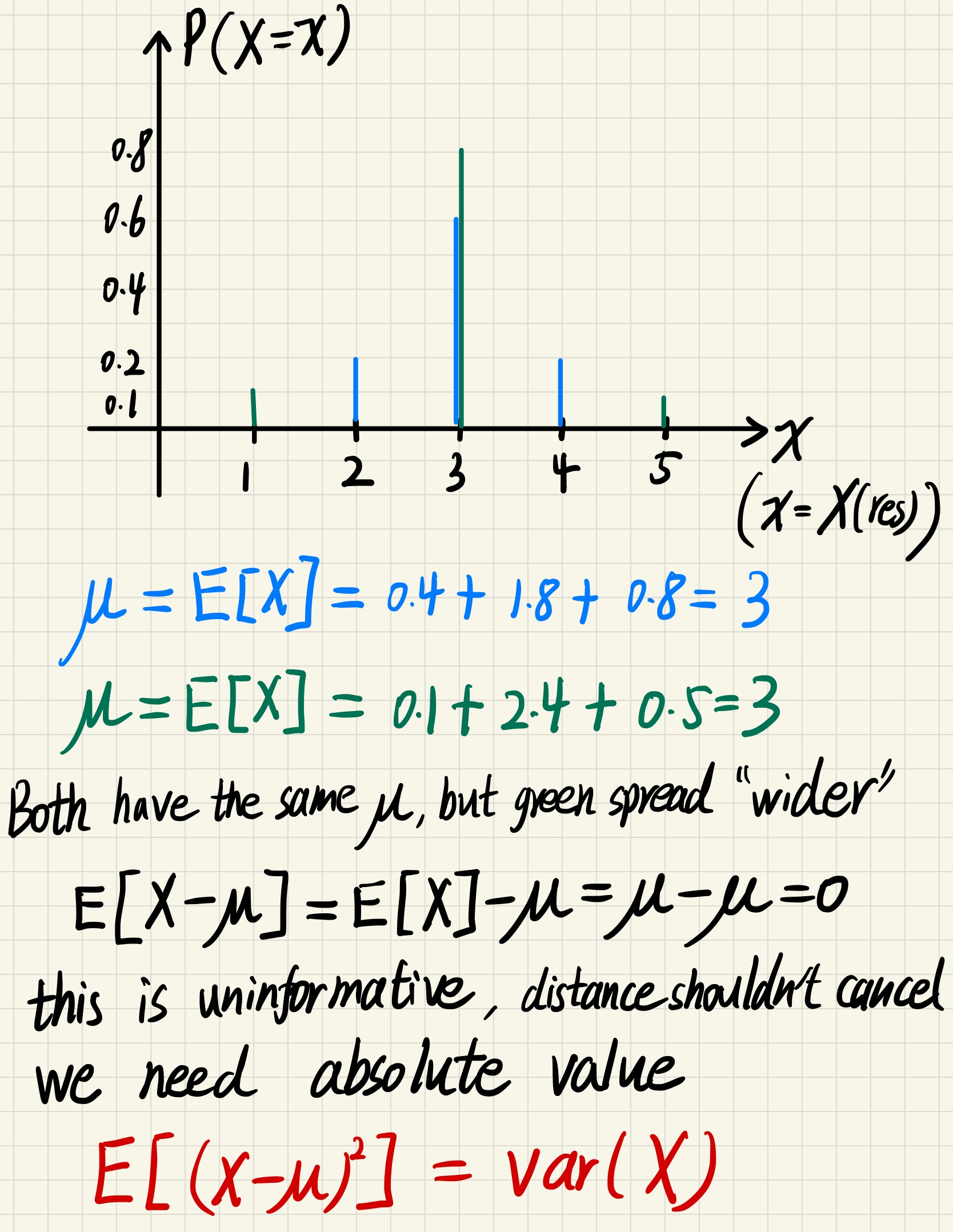
$$
var(X) = E[(X-\mu)^2] = E[g(X)] = \sum g(x)P_X(x)
$$

Property of variance

$$
var(aX+b) = a^2var(X)
$$

$$
var(X+b)= E[(X+b-(\mu+b))^2] = E[(X-\mu)^2] = var(X)
$$

(just moving the graph left/right by the const $b$, distance won’t change)

$$
var(aX) = E[(aX-a\mu)^2] = E[a^2(X-\mu)^2] = a^2var(X)
$$

A useful formula, quick calculation

$$
var(X) = E[X^2]-(E[X])^2
$$

$$
\because var(X) = E[(X-\mu)^2]
$$

$$
= \sum X^2P_X(x) - 2\mu\sum XP_X(x) + \mu^2
$$

$$
= E[X^2] - 2\mu^2 + \mu = E[X^2]-(E(X)^2)
$$

Example

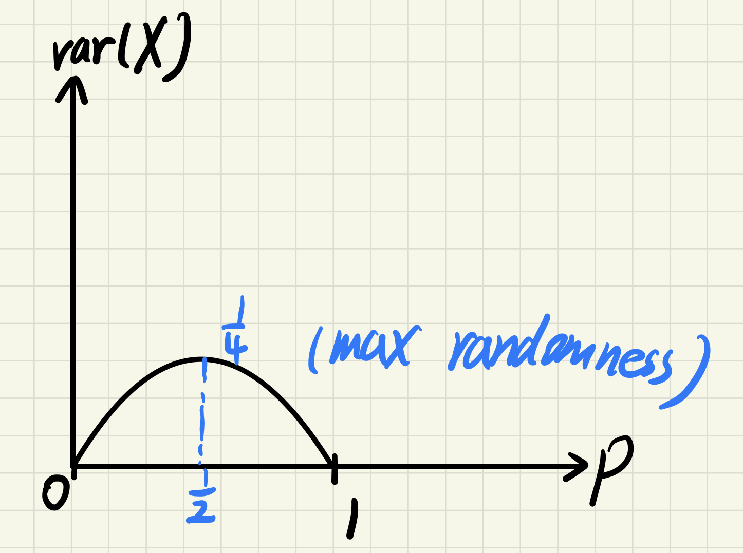
variance indicate the randomness of a PMF, larger variance gives larger randomness

Bernoulli variance

$$
var(X) = p(1-p)
$$

A coin is most random when it is fair.

Conditional PMF

Total expectation theorem

Multiple r.v. and joint PMF

Joint PMF

$$
P_{X,Y} (x,y) = P(X=x \land Y = y)
$$

• $\sum_{\text{all x}}\sum_{\text{all y}}P_{X,Y}(x,y)=1$

• $P_X(x) = \sum_\text{all y} P_{X,Y}(x,y)$

• $E[g(X,Y)] = \sum_\text{all x}\sum_\text{all y} g(x,y)P_{X,Y}(x,y)$

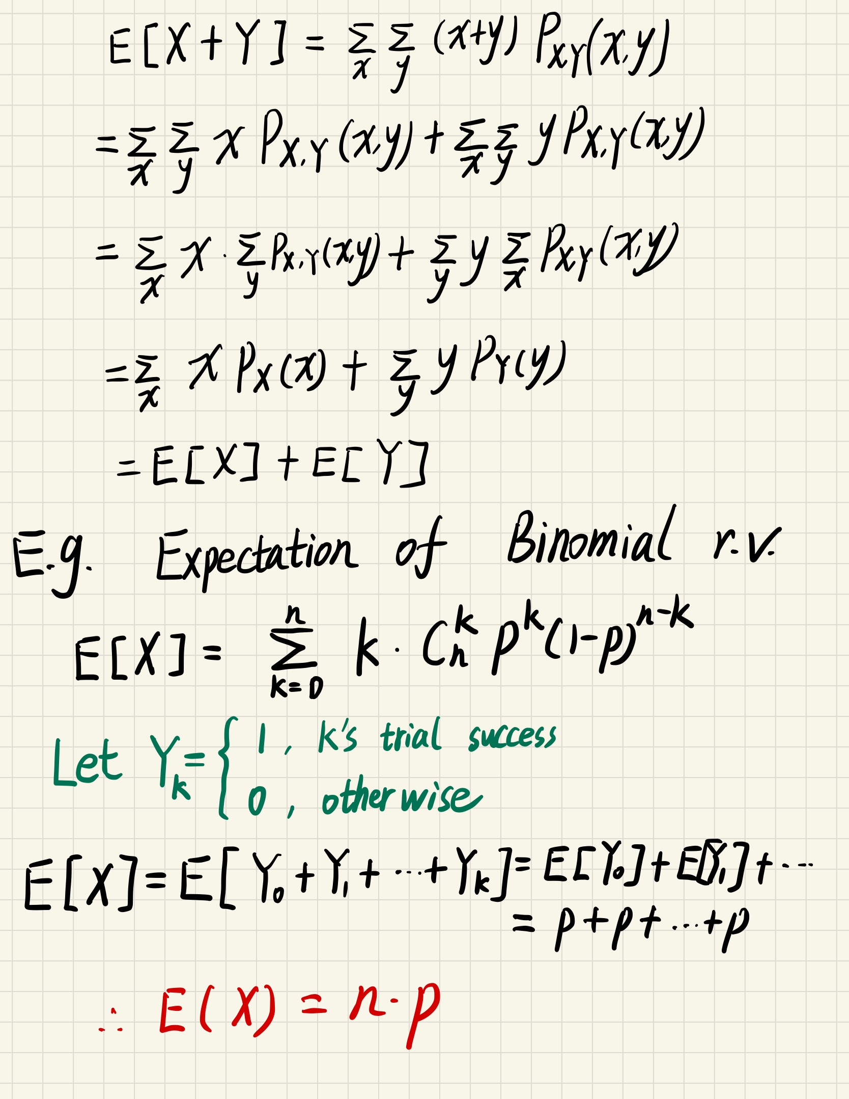
• $E[X+Y] = E[X]+E[Y]$

Independent r.v.

$$
P_{X|Y}(x,y) = P(X=x | Y=y) = \frac{P( X=x \land Y = y )}{P(Y=y)}
$$

$$
= \frac{P_{X,Y}(x,y)}{P_Y(y)}
$$

And for every $y$, we take it as if it is a const

$$
\sum_\text{for all x} P_{X|Y}(x,y) = 1
$$

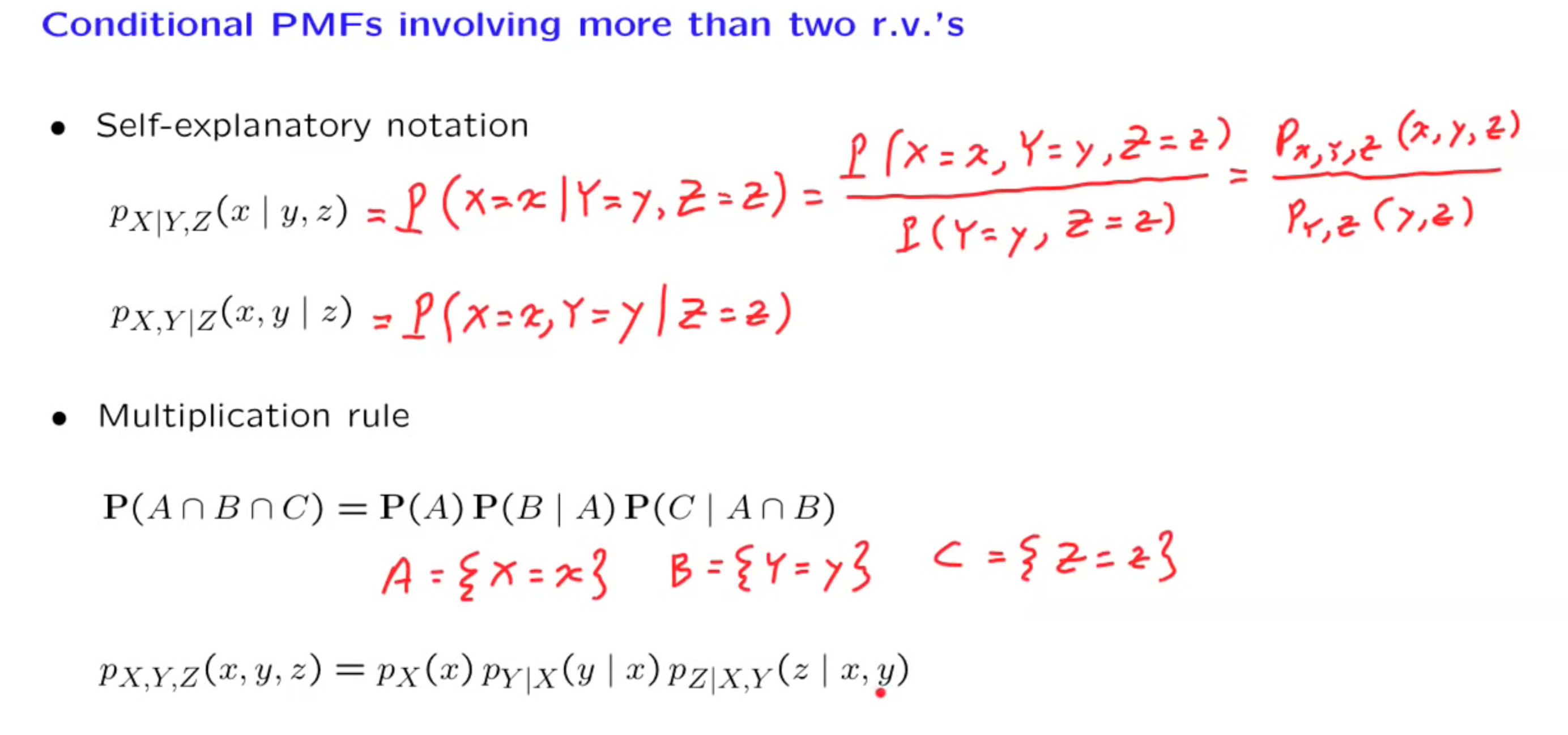
Multiplication rule for conditioning r.v.

$$
P_{X|Y}(x,y) = P_{Y}(y) \times P_{X|Y}(x|y)
$$

Total Probability theorem

$$
P_X(x) = \sum_\text{all y}P_Y(y)P_{X|Y}(x|y)
$$

Total Expectation theorem

$$
E[X] = \sum_\text{all y} P_Y(y)E[X|Y=y]
$$

$$
E[X|Y=y] = \sum_\text{all y}x \times P_{X|Y}(x|y)
$$

Independent r.v.

Similar with independent events

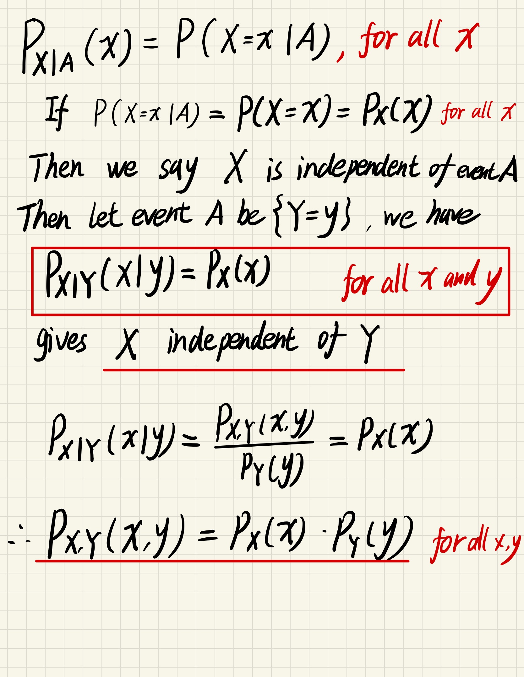
$$
P_{X,Y,Z}(x,y,z)=P_X(x)P_Y(y)P_Z(z)
$$

The random variables are independent when they do not intersect with each other, knowing any probability of any random variable will give any information about the probability of the rest r.v.

jointPMF == functools.reduce( lambda x,y : x*y , marginalPMFs )

Independent expectation

$$
X \text{ and } Y \text{ are independent} \implies E[XY] = E[X]E[Y]
$$

$$
E[XY] = \sum_{x}\sum_{y}xyP_{X,Y}(x,y)
$$

$$
\because P_{X,Y}(x,y) = P_X(x)P_Y(y)
$$

$$
\therefore \sum_{x}\sum_{y}xyP_{X,Y}(x,y) = \sum_{x}\sum_{y}xP_{X}(x)yP_Y(y)
$$

$$
= \sum_xxP_{X}(x)\sum_yyP_Y(y) = \sum_xP_X(x)E[Y]
$$

$$
= E[Y] \sum_xP_X(x) = E[Y]E[X]
$$

And this can expand to more situations

$$
E[g(X)h(Y)]= E[g(X)]E[h(Y)]
$$

Independent variance

$$
X \text{ and } Y \text{ are independent} \implies var(X+Y) = var(X) + var(Y)
$$

Example

variance of binomial r.v.

same trick when calculating expectation

$$
var(X)= var(X_1 + X_2 + … +X_i) = var(X_1)+var(X_2)+…
$$

$$
= n\times var(X_1) = n p(1-p)
$$