Continuous Random Variable

Let calculus in

Probability density function(PDF)

PMF in continuous situation

Continuous set is NOT enough, it must be able to be describe by a PDF

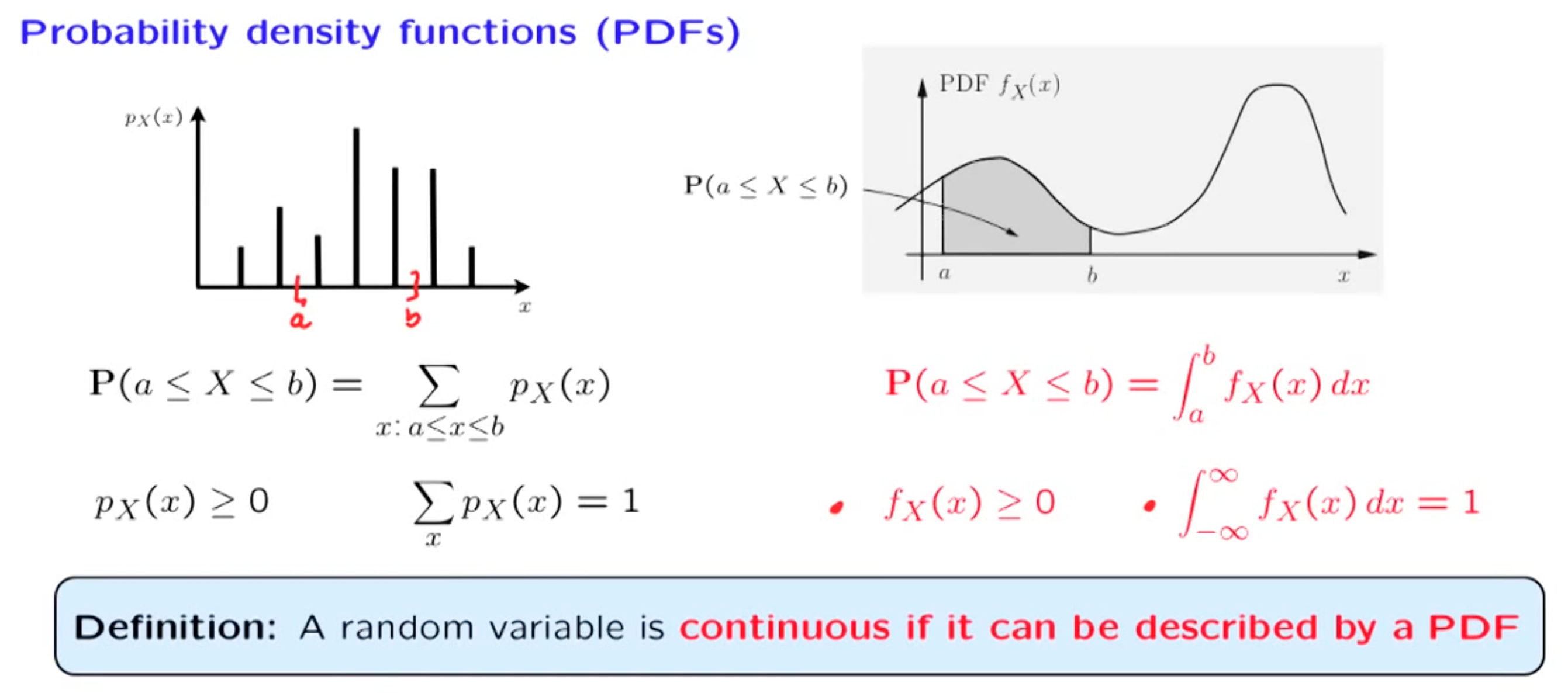
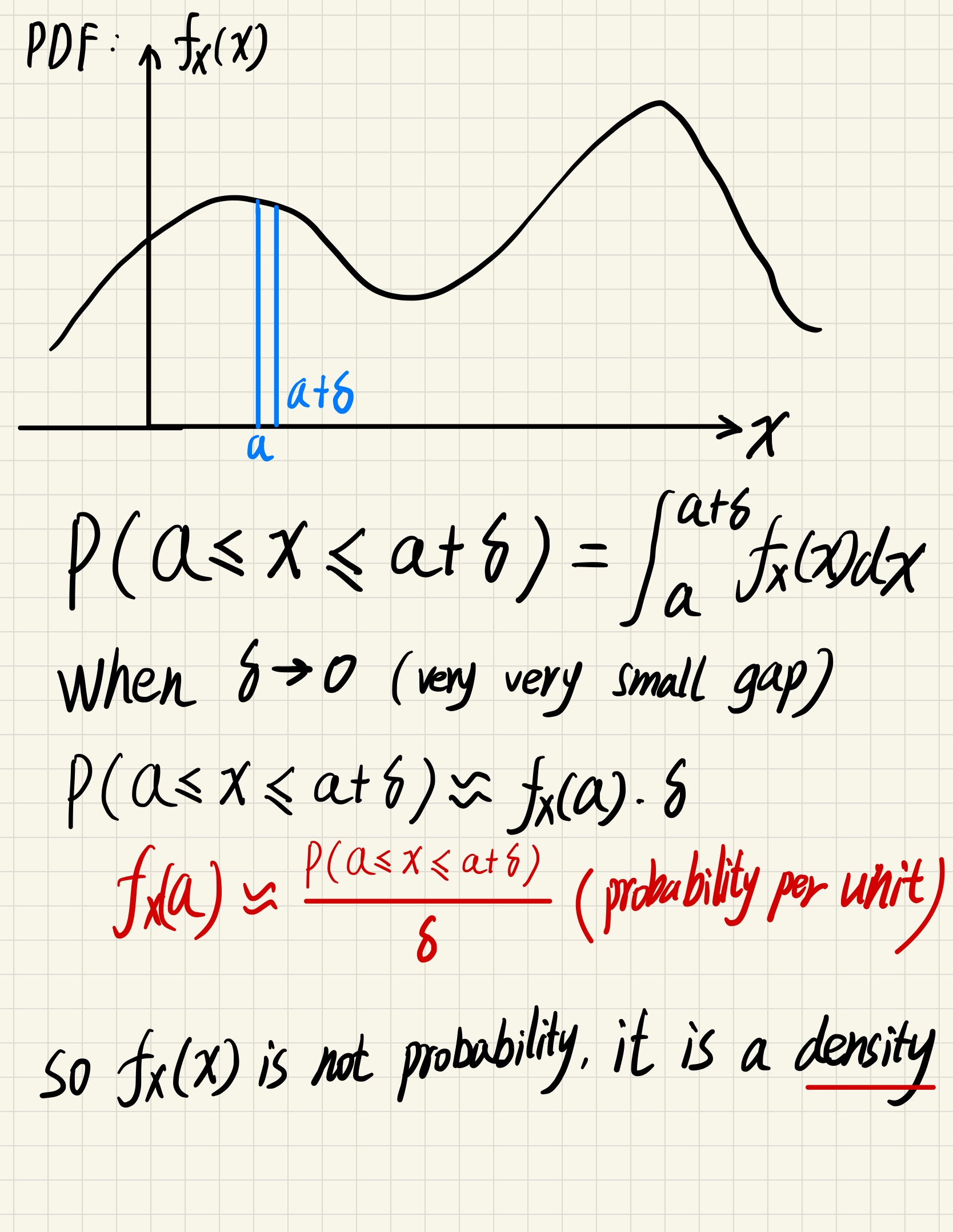
The area is the probability, height only denote density

For any given point $a$, $f_X(a) = 0$

$$
\because P(a \le x \le b) = P(x=a)+P(a < x < b) + P(x=b)
$$

$$
\therefore P(a\le x \le b) = P(a < x < b)
$$

(We don’t care about endpoints)

(Single point do not have length, infinite number of points will have a length, this is same for probability density)

Expectation

$$
E[X] = \int_{-\infty}^\infty x f_X(x) dx
$$

Don’t forget that the expectation equals to the “balance point”, for symmetric ones, it is the center point.

Exponential Random Variable

$$
f_X(x) = \begin{cases}
\lambda e ^{-\lambda x} ,& x \ge 0\
0, & x < 0
\end{cases}, \text{parameter} \lambda > 0
$$

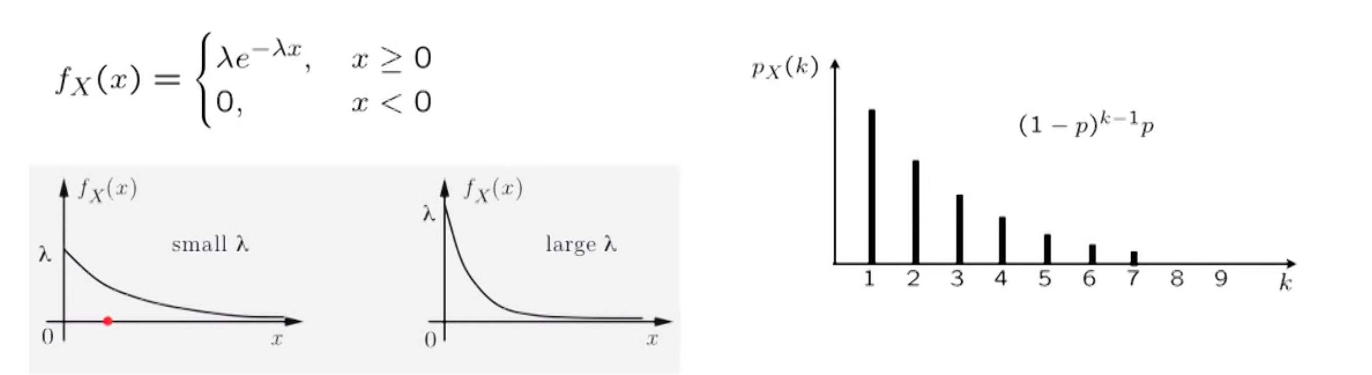
We can see that exponential distribution is similar to geometry distribution in discrete case.

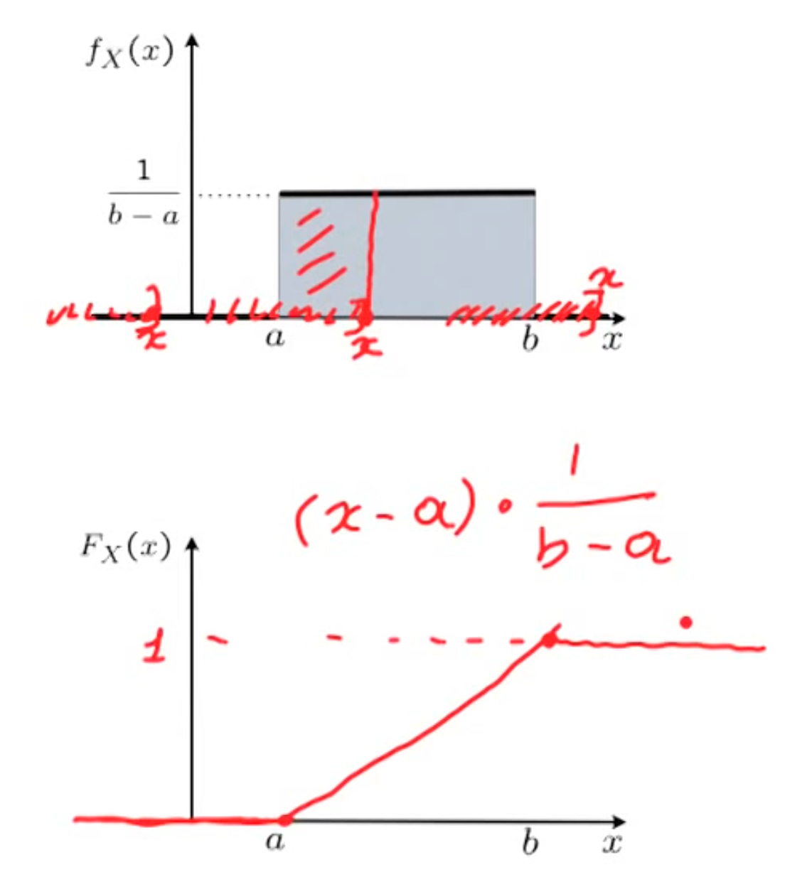
Cumulative Distribution Function(CDF)

another beautiful way for describing random variables

$$
F_X(x) = P(X \le x)
$$

Continuous

integral and derivative

$$
F_X(x) = \int_{-\infty}^{x} f_X(x)dx
$$

Discrete

$$
F_X(x) = \sum _ \text{all k less than x} P_X(k)
$$

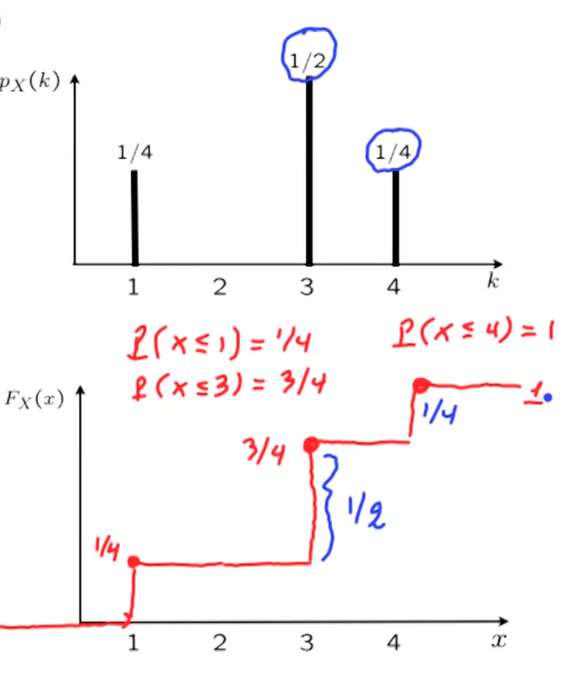
Property

• non-decrease, CDF is “accumulative”

• CDF goes to 1 as x approaching plus infinity

• CDF goes to 0 as x approaching minus infinity

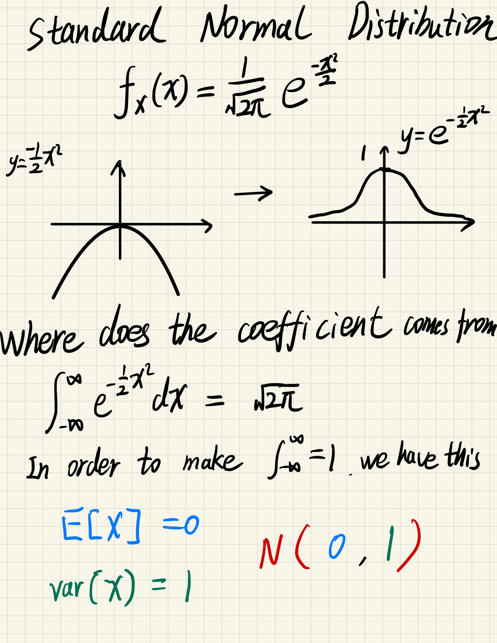
Normal(Gaussian) Distribution

Standard Normal

$$
N(0,1) : f_X(x) = \frac{1}{\sqrt{2\pi}} e^\frac{-x^2}{2}
$$

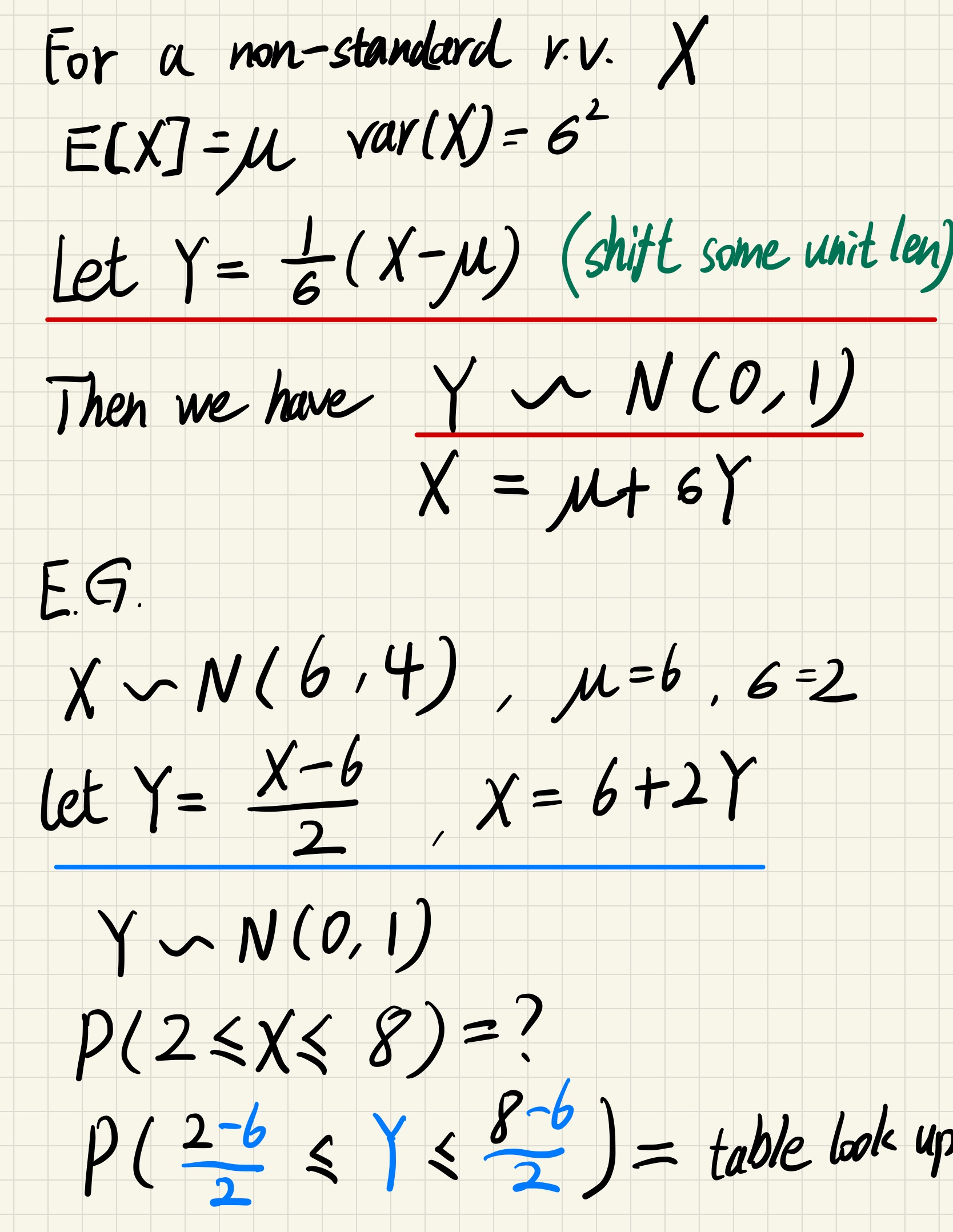
General Normal

$$
N(\mu , \sigma^2 ) : f_X(x) = \frac{1}{\sigma \sqrt{2\pi}} e ^{\frac{-(x-\mu)^2}{2\sigma^2}}
$$

Linear form

when we apply a linear form to the random variable, normal distribution is preserved

$$
X \sim N(\mu , \sigma^2)
$$

$$
Y = aX+b
$$

$$
then , Y \sim N(a\mu + b , a^2\sigma^2)
$$

Standardize a random variable

just moving the axis

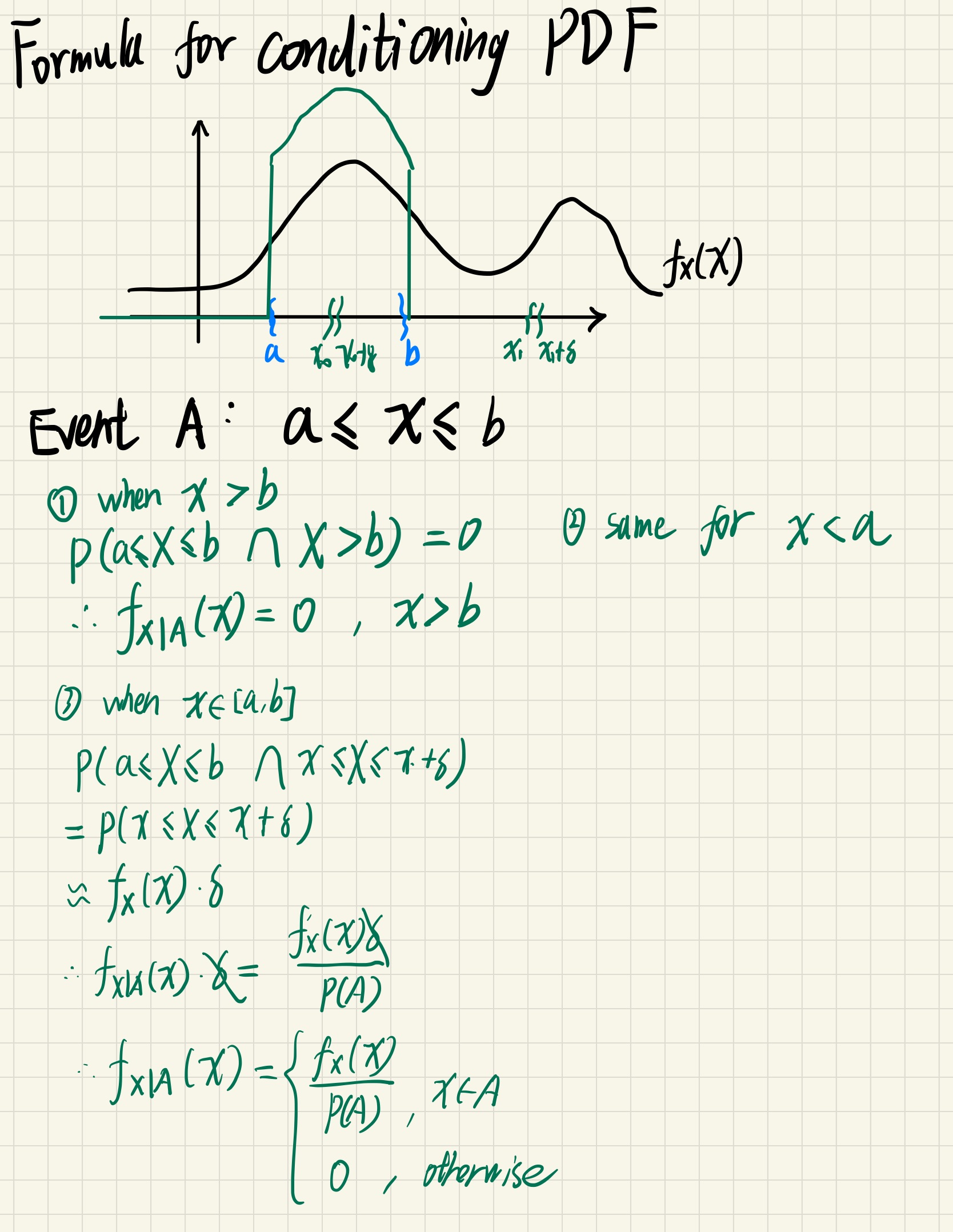
Conditioning continuous r.v.

only some addition information provided, stick to the definition

Memoryless property

the light bulb won’t remember what has happened, they appear as completely new!

Example

Two light bulb to choose : the first one has been working for $t$ time, the second one is completely new, which one to choose ? (Every light bulb has a life time $T$, exponential model)

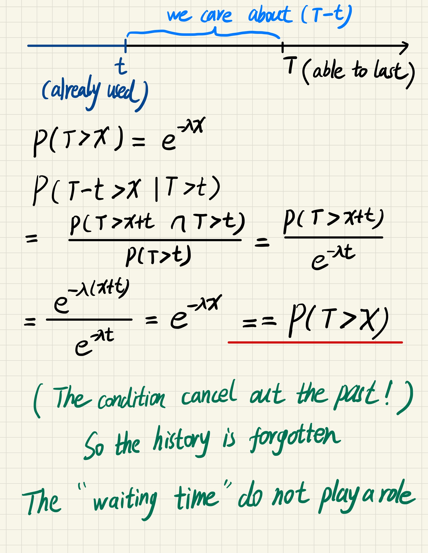
It usually refers to the cases when the distribution of a “waiting time” until a certain event does not depend on how much time has elapsed already.

To model memoryless situations accurately, we must constantly ‘forget’ which state the system is in: the probabilities would not be influenced by the history of the process.

Only two kinds of distributions are memoryless: geometric distributions of non-negative integers and the exponential distributions of non-negative real numbers.

(We can also view exponential distribution as the continuous case for geometric distribution)

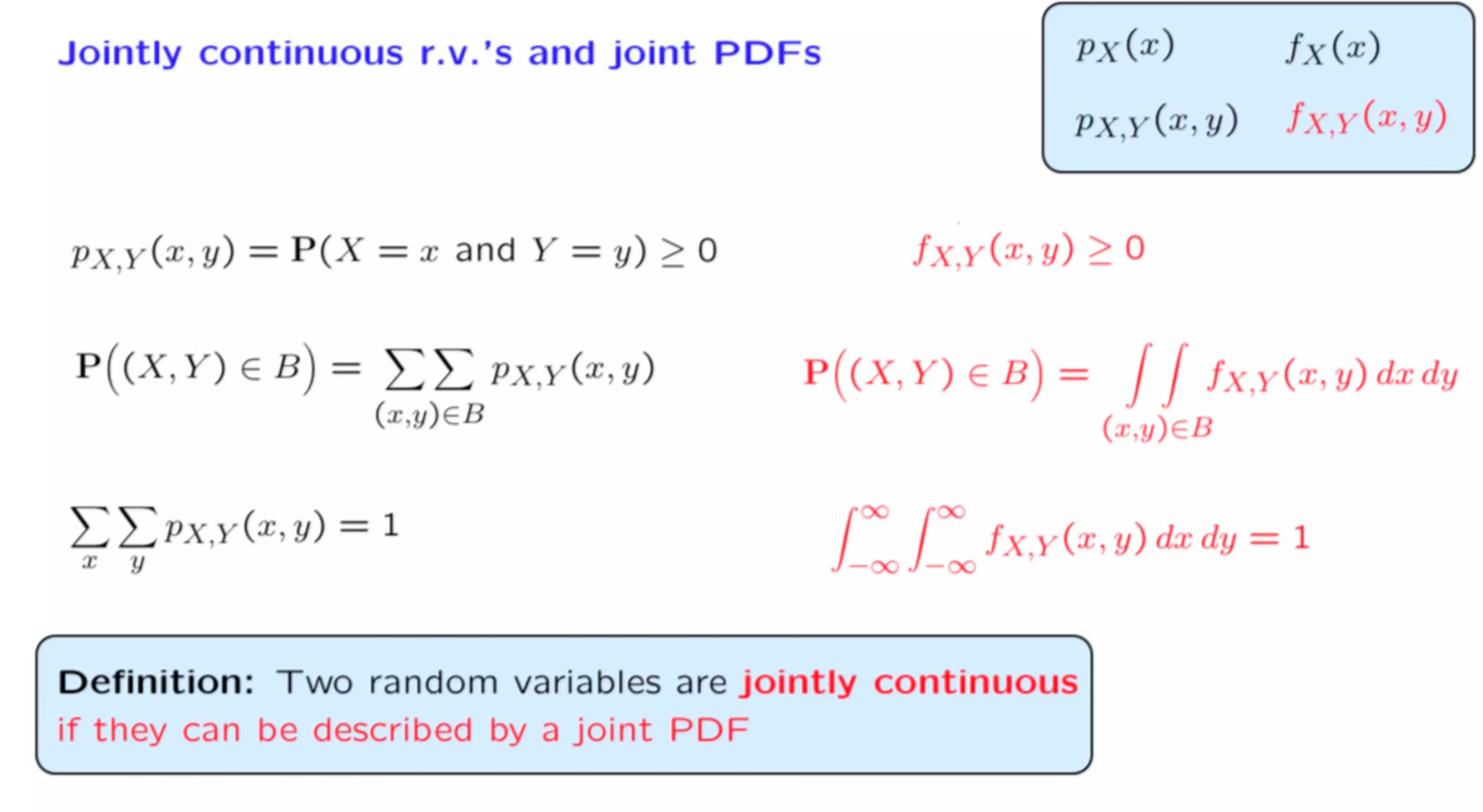
Joint PDF

This is just a definition, we define it to be this way without special meaning

(From geometric view, joint PDF is the probability of per unit area, the “height”)

Conditioning PDF

a slice of joint PDF

$$
P(X=x | Y = y) =\frac{P(X = x \land Y = y)}{P(Y=y)}
$$

However, in continuous situation, the denominator will always be 0. So we mimic the formula and gives a conditioning definition.

$$
P( x \le X \le x + \delta | y \le Y \le y + \epsilon ) = \frac{f_{X,Y}(x,y)\delta\epsilon}{f_Y(y)\epsilon}
$$

$$
let \ \frac{f_{X,Y}(x,y)}{f_Y(y)} = f_{X|Y}(x|y)
$$

Multiplication Rule

$$
f_{X,Y}(x,y) = f_Y{(y)}f_{X|Y}(x|y) = f_X(x)f_{Y|X}(y|x)
$$

Total Probability Theorem

$$
f_{X}(x) = \int_{-\infty}^\infty f_Y(y) f_{X|Y}(x|y)dy
$$

Independence

one variable does not provide any information for another

$$
f_{X,Y}(x,y) = f_X(x)f_Y(y)
$$

$$
f_{X,Y}(x,y) = f_Y{(y)}f_{X|Y}(x|y) \implies f_X(x)=f_{X|Y}(x|y)
$$

Bayes’ rule

We want to infer the environment via occurred events

$$
f_{X|Y}(x|y) = \frac{f_X(x)f_{Y|X}(y|x)}{ \int f_X(x)f_{Y|X}(y|x) dx }
$$